For full references, please refer to: https://dhlab-tseng.github.io/lab/index.html

lab
I. Introduction
The proposed open-source lab package is a software tool that help users to explore and process laboratory data in electronic health records (EHRs). With the lab package, researchers can easily map local laboratory codes to the universal standard, mark abnormal results, summarize data using descriptive statistics, impute missing values, and generate analysis ready data.
Feature
- Data Mapping Standardize and manipulate data with Logical Observation Identifiers Names and Codes (LOINC), a common terminology for laboratory and clinical observations.
- Time Series Analysis Separate lab test results into multiple consecutive non-overlapped time windows
- Value Imputation Impute value to replace missing data
- Wide Format Generation Transform longitudinal data into wide format to generate analysis ready data
Development version
# install.packages("remotes")
remotes::install_github("DHLab-TSENG/lab")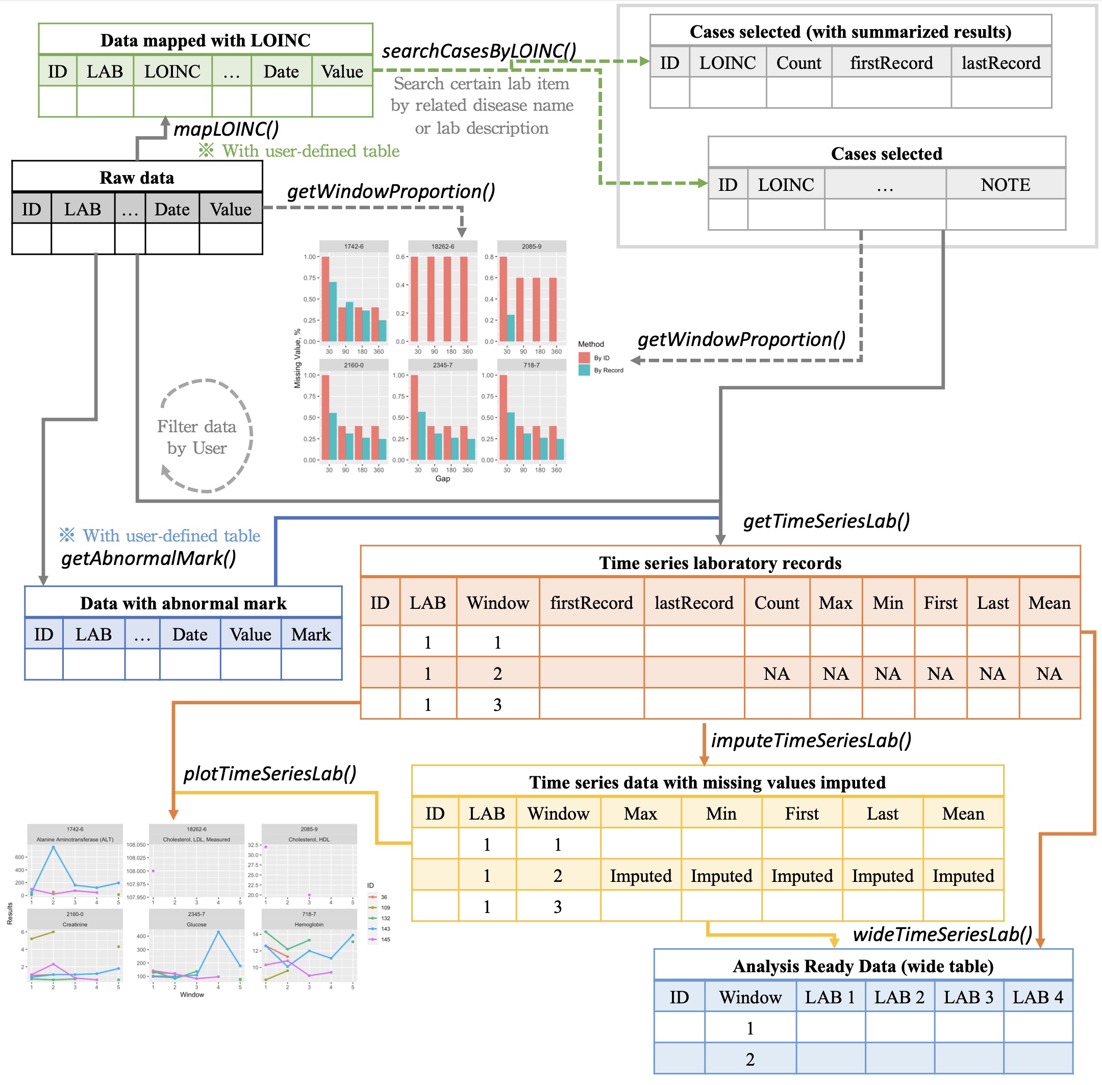
Usage
# install.packages("remotes")
remotes::install_github("DHLab-TSENG/lab")
library(lab)
Dataset
The sample data includes 1,744 lab records containing 7 different lab items tested by 5 patients from MIMIC-III database.
head(labSample)
#>    SUBJECT_ID ITEMID  CHARTTIME VALUENUM VALUEUOM     FLAG
#> 1:         36  50811 2131-05-18     12.7     g/dL abnormal
#> 2:         36  50912 2131-05-18      1.2    mg/dL
#> 3:         36  51222 2131-05-18     11.9     g/dL abnormal
#> 4:         36  50912 2131-05-19      1.3    mg/dL abnormal
#> 5:         36  50931 2131-05-19    160.0    mg/dL abnormal
#> 6:         36  51222 2131-05-19      9.6     g/dL abnormal
I. Data Mapping
If LOINC is not the default terminology, users are recommended to map local lab item with LOINC by providing mapping table.
First, user shall prepare a mapping table with local codes and LOINC codes.
head(mapSample)
#>    ITEMID                          LABEL FLUID  CATEGORY   LOINC
#> 1:  50811                     Hemoglobin Blood Blood Gas   718-7
#> 2:  50861 Alanine Aminotransferase (ALT) Blood Chemistry  1742-6
#> 3:  50904               Cholesterol, HDL Blood Chemistry  2085-9
#> 4:  50906     Cholesterol, LDL, Measured Blood Chemistry 18262-6
#> 5:  50912                     Creatinine Blood Chemistry  2160-0
#> 6:  50931                        Glucose Blood Chemistry  2345-7
loincSample <- mapLOINC(labData = labSample, labItemColName = ITEMID, mappingTable = mapSample)

head(loincSample)
#>    ITEMID SUBJECT_ID  CHARTTIME VALUENUM VALUEUOM     FLAG      LABEL FLUID
#> 1:  50811         36 2131-05-18     12.7     g/dL abnormal Hemoglobin Blood
#> 2:  50811         36 2131-05-04     12.3     g/dL abnormal Hemoglobin Blood
#> 3:  50811         36 2131-05-15     10.0     g/dL abnormal Hemoglobin Blood
#> 4:  50811         36 2131-05-17     11.7     g/dL abnormal Hemoglobin Blood
#> 5:  50811        109 2142-02-25      6.9     g/dL abnormal Hemoglobin Blood
#> 6:  50811        109 2141-09-20      7.2     g/dL abnormal Hemoglobin Blood
#>     CATEGORY LOINC
#> 1: Blood Gas 718-7
#> 2: Blood Gas 718-7
#> 3: Blood Gas 718-7
#> 4: Blood Gas 718-7
#> 5: Blood Gas 718-7
#> 6: Blood Gas 718-7
Once a user map lab test codes with LOINC, ranges can be used to mark abnormal results, and related names can be used to search related lab test codes by other common names of a lab test.
loincMarkedSample <- getAbnormalMark(labData = loincSample,
                                     idColName = SUBJECT_ID,
                                     labItemColName = LOINC,
                                     valueColName = VALUENUM,
                                     genderColName = GENDER,
                                     genderTable = patientSample,
                                     referenceTable = refLOINC)
head(loincMarkedSample)
#>    ITEMID  ID  CHARTTIME Value VALUEUOM     FLAG                          LABEL
#> 1:  50861  36 2131-04-30     8     IU/L          Alanine Aminotransferase (ALT)
#> 2:  50861  36 2131-05-17    12     IU/L          Alanine Aminotransferase (ALT)
#> 3:  50861  36 2134-05-14    12     IU/L          Alanine Aminotransferase (ALT)
#> 4:  50861 109 2138-07-03    14     IU/L          Alanine Aminotransferase (ALT)
#> 5:  50861 109 2142-03-21    46     IU/L abnormal Alanine Aminotransferase (ALT)
#> 6:  50861 109 2142-01-09    10     IU/L          Alanine Aminotransferase (ALT)
#>    FLUID  CATEGORY  LOINC ABMark
#> 1: Blood Chemistry 1742-6   <NA>
#> 2: Blood Chemistry 1742-6   <NA>
#> 3: Blood Chemistry 1742-6   <NA>
#> 4: Blood Chemistry 1742-6   <NA>
#> 5: Blood Chemistry 1742-6      H
#> 6: Blood Chemistry 1742-6   <NA>
caseCreatinine <- searchCasesByLOINC(labData = loincSample,
                                     idColName = SUBJECT_ID,
                                     loincColName = LOINC,
                                     dateColName = CHARTTIME,
                                     condition = "Creatinine",
                                     isSummary = TRUE)

head(caseCreatinine)
#>     ID  LOINC Count firstRecord lastRecode
#> 1:  36 2160-0    37  2131-04-30 2134-05-20
#> 2: 109 2160-0   238  2137-11-04 2142-08-30
#> 3: 132 2160-0    32  2115-05-06 2116-04-08
#> 4: 143 2160-0    60  2154-12-25 2155-10-22
#> 5: 145 2160-0   162  2144-03-29 2145-02-22
II. Time Series Analysis
lab package allows users to separate lab test results into multiple consecutive non-overlapped time windows. The index date of time windows can be the first or last event occurred for individuals, or a specific date for all patients. To help users find suitable window size (e.g., 30 days or 180 days, to name but a few), a plot function is provided to visualize how frequent the patients did each lab test.
windowProportion <- plotWindowProportion(labData = loincSample,
                                         idColName = SUBJECT_ID,
                                         labItemColName = LOINC,
                                         dateColName = CHARTTIME,
                                         indexDate = first,
                                         gapDate = c(30, 90, 180, 360),
                                         studyPeriodStartDays=0,
                                         studyPeriodEndDays=360)

print(windowProportion$graph)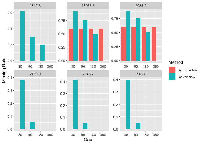
head(windowProportion$missingData)
#>       LAB Gap        Method Proportion
#> 1: 1742-6  30 By Individual          0
#> 2: 1742-6  30 By Individual          0
#> 3: 1742-6  30 By Individual          0
#> 4: 1742-6  30 By Individual          0
#> 5: 1742-6  30 By Individual          0
#> 6: 2160-0  30 By Individual          0
After the index date and window size are decided, the descriptive statistics information, including total test times within a window, maximum test value, minimum test value, test values average, and the record nearest to the index date, are shown.
timeSeriesData <- getTimeSeriesLab(labData = loincSample,
                                   idColName = SUBJECT_ID,
                                   labItemColName = LOINC + LABEL,
                                   dateColName = CHARTTIME,
                                   valueColName = VALUENUM,
                                   indexDate = first,
                                   gapDate = 30,
                                   completeWindows = TRUE)
head(timeSeriesData)
#>    ID  LOINC                          LABEL Window Count Max Min Mean Nearest
#> 1: 36 1742-6 Alanine Aminotransferase (ALT)      1     2  12   8   10       8
#> 2: 36 1742-6 Alanine Aminotransferase (ALT)      2    NA  NA  NA   NA      NA
#> 3: 36 1742-6 Alanine Aminotransferase (ALT)      3    NA  NA  NA   NA      NA
#> 4: 36 1742-6 Alanine Aminotransferase (ALT)      4    NA  NA  NA   NA      NA
#> 5: 36 1742-6 Alanine Aminotransferase (ALT)      5    NA  NA  NA   NA      NA
#> 6: 36 1742-6 Alanine Aminotransferase (ALT)      6    NA  NA  NA   NA      NA
#>    firstRecord lastRecode
#> 1:  2131-04-30 2131-05-17
#> 2:        <NA>       <NA>
#> 3:        <NA>       <NA>
#> 4:        <NA>       <NA>
#> 5:        <NA>       <NA>
#> 6:        <NA>       <NA>
Also, a line chart plotting function is available to do long-term follow-up. Visualization is helpful for detecting data trends. Additionally, “L” and “H” will be used as legendary icon if abnormal values are marked.
timeSeriesPlot <- plotTimeSeriesLab(labData = timeSeriesData,
                                    idColName = ID,
                                    labItemColName = LOINC + LABEL,
                                    timeMarkColName = Window,
                                    valueColName = Nearest,
                                    timeStart = 1,
                                    timeEnd  = 5,
                                    abnormalMarkColName = NULL)

plot(timeSeriesPlot)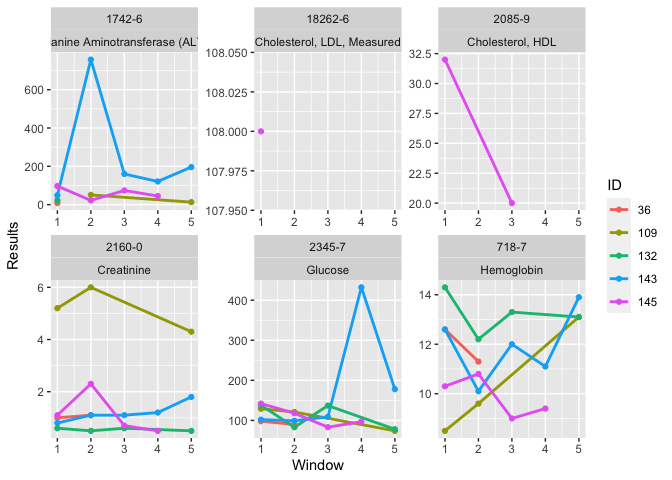
III. Imputation
Imputation function can be executed to replace missing data.
fullTimeSeriesData <- imputeTimeSeriesLab(labData = timeSeriesData,
                                          idColName = ID,
                                          labItemColName = LOINC + LABEL,
                                          windowColName = Window,
                                          valueColName = Mean & Nearest,
                                          impMethod = NOCB,
                                          imputeOverallMean = FALSE)
fullTimeSeriesData[timeSeriesData$ID==36&
                     timeSeriesData$LOINC=="2160-0"]
#>     ID  LOINC      LABEL Window      Mean Nearest imputed
#>  1: 36 2160-0 Creatinine      1 1.2347826     1.0   FALSE
#>  2: 36 2160-0 Creatinine      2 1.1000000     1.1   FALSE
#>  3: 36 2160-0 Creatinine      3 1.1000000     1.1    TRUE
#>  4: 36 2160-0 Creatinine      4 1.1000000     1.1    TRUE
#>  5: 36 2160-0 Creatinine      5 1.1000000     1.1    TRUE
#>  6: 36 2160-0 Creatinine      6 1.1000000     1.1    TRUE
#>  7: 36 2160-0 Creatinine      7 1.1000000     1.1    TRUE
#>  8: 36 2160-0 Creatinine      8 1.1000000     1.1    TRUE
#>  9: 36 2160-0 Creatinine      9 1.2000000     1.2   FALSE
#> 10: 36 2160-0 Creatinine     10 1.1000000     1.1   FALSE
#> 11: 36 2160-0 Creatinine     11 1.1000000     1.1    TRUE
#> 12: 36 2160-0 Creatinine     12 1.1000000     1.1    TRUE
#> 13: 36 2160-0 Creatinine     13 1.1000000     1.1    TRUE
#> 14: 36 2160-0 Creatinine     14 1.1000000     1.1    TRUE
#> 15: 36 2160-0 Creatinine     15 1.1000000     1.1    TRUE
#> 16: 36 2160-0 Creatinine     16 1.1000000     1.1    TRUE
#> 17: 36 2160-0 Creatinine     17 1.1000000     1.1    TRUE
#> 18: 36 2160-0 Creatinine     18 1.1000000     1.1    TRUE
#> 19: 36 2160-0 Creatinine     19 1.1000000     1.1    TRUE
#> 20: 36 2160-0 Creatinine     20 1.1000000     1.1    TRUE
#> 21: 36 2160-0 Creatinine     21 1.1000000     1.1    TRUE
#> 22: 36 2160-0 Creatinine     22 1.1000000     1.1    TRUE
#> 23: 36 2160-0 Creatinine     23 1.1000000     1.1    TRUE
#> 24: 36 2160-0 Creatinine     24 1.1000000     1.1    TRUE
#> 25: 36 2160-0 Creatinine     25 1.1000000     1.1    TRUE
#> 26: 36 2160-0 Creatinine     26 1.1000000     1.1    TRUE
#> 27: 36 2160-0 Creatinine     27 1.1000000     1.1    TRUE
#> 28: 36 2160-0 Creatinine     28 1.1000000     1.1    TRUE
#> 29: 36 2160-0 Creatinine     29 1.1000000     1.1    TRUE
#> 30: 36 2160-0 Creatinine     30 1.1000000     1.1    TRUE
#> 31: 36 2160-0 Creatinine     31 1.1000000     1.1    TRUE
#> 32: 36 2160-0 Creatinine     32 1.1000000     1.1    TRUE
#> 33: 36 2160-0 Creatinine     33 1.1000000     1.1    TRUE
#> 34: 36 2160-0 Creatinine     34 1.1000000     1.1    TRUE
#> 35: 36 2160-0 Creatinine     35 1.1000000     1.1    TRUE
#> 36: 36 2160-0 Creatinine     36 1.1000000     1.1    TRUE
#> 37: 36 2160-0 Creatinine     37 0.9666667     1.0   FALSE
#> 38: 36 2160-0 Creatinine     38 0.8500000     0.9   FALSE
#>     ID  LOINC      LABEL Window      Mean Nearest imputed
IV. Wide Format Generation
Then, a function be used to transform longitudinal data into wide format to generate analysis ready data.
wideTimeSeriesData <- wideTimeSeriesLab(labData = fullTimeSeriesData,
                                        idColName = ID,
                                        labItemColName = LOINC + LABEL,
                                        windowColName = Window,
                                        valueColName = Nearest)
head(wideTimeSeriesData)
#>    ID Window 1742-6_Alanine Aminotransferase (ALT)
#> 1: 36      1                                     8
#> 2: 36      2                                     8
#> 3: 36      3                                     8
#> 4: 36      4                                     8
#> 5: 36      5                                     8
#> 6: 36      6                                     8
#>    18262-6_Cholesterol, LDL, Measured 2085-9_Cholesterol, HDL 2160-0_Creatinine
#> 1:                                 NA                      NA               1.0
#> 2:                                 NA                      NA               1.1
#> 3:                                 NA                      NA               1.1
#> 4:                                 NA                      NA               1.1
#> 5:                                 NA                      NA               1.1
#> 6:                                 NA                      NA               1.1
#>    2345-7_Glucose 718-7_Hemoglobin
#> 1:             98             12.6
#> 2:             90             11.3
#> 3:             90             11.3
#> 4:             90             11.3
#> 5:             90             11.3
#> 6:             90             11.3