Getting started with dxtime
Yi-An, Zhu
2021-09-07
dxtime.Rmd安裝套件
install.packages("devtools")
devtools::install_github("DHLab-TSENG/dxtime")
library(dxtime)
範例資料
以下功能介紹皆以pat_dm以及record_dm做為範例。
pat_dm中共200名個案,170位病例組(label=1),30位為對照組(label=0);
record_dm為該200名個案在指標日(發生疾病/最後一筆…)的之診斷紀錄。
head(pat_dm)
#>    ID   birthday gender label age
#> 1:  1 1956-03-18      F     0  50
#> 2:  2 1976-04-26      M     0  42
#> 3:  3 1950-06-02      M     0  68
#> 4:  4 1984-10-21      M     0  33
#> 5:  5 1944-08-01      M     0  74
#> 6:  6 1982-11-27      M     0  32
head(record_dm)
#>     ID       date  ICD dataLength
#> 1: 149 2015-07-08 4019  6077 days
#> 2: 149 2015-07-08 2720  6077 days
#> 3: 149 2015-07-08 7840  6077 days
#> 4: 149 2015-09-30 4019  6077 days
#> 5: 149 2015-09-30 2720  6077 days
#> 6: 149 2015-09-30 7840  6077 days
使用流程
名詞在時間軸上狀態 
一、篩選符合研究長度之個案及診斷紀錄
在病例對照研究,會探討回溯期間內的暴露因子與疾病發生的關係。隨著回溯時間長度越長,所囊括的暴露的危險因子會越多,樣本比較之下,將會造成「回溯時長較長的樣本,危險因子較多」的偏誤。
為避免這種偏誤,固定追蹤時長是較佳的作法。但每個樣本的發病日期(indexDate)並不相同,在filterCasesRecords()可回推追蹤時間,找出追蹤時間範圍內的診斷資料;此外,資料長度不足的樣本也可將之排除。
主要需設定的參數有:predictGap: 預測天數,意指「想要於指標日多久前進行預測」。exposurePeriod:此研究所設定的危險因子暴露時長,將用於篩選時間範圍內的診斷紀錄。includePeriodAtLeast:病患須擁有的資料長度下限。結果將依設定將資料長度不足的個案於以排除,預設為0。countICDAtLeast:病患須擁有的資料筆數下限,若是診斷紀錄的筆數過少,有可能意味著該個案極少至此醫療單位看診,研究者可設定診斷紀錄的數量下限,來決定是否採納此個案之紀錄,預設為0。align:設定納入資料的方式,是由起始點往後(align=“left”),或是預測點往回推(align=“right”),預設為right。
執行結束會產生兩種結果,分別是Patient(病患資料)及Record(診斷資料)。
#dxData <- merge(record_dm,pat_dm[,c("ID","label")],by="ID",all.x=T)
length <- filterCasesRecords(DataFile = record_dm,
                             idColName = ID,
                             icdColName = ICD,
                             dateColName = date,
                             predictGap = 180,
                             exposurePeriod = 1800,
                             includePeriodAtLeast = 360,
                             countICDAtLeast = 2,
                             align="right"
                             )
以上框結果說明:
第一種結果Patient,該資料表顯示三個時間點,firstDate、predicDate、indexDate。 firstDate為第一筆診斷紀錄的日期;predictDate為預測資料的最後一個預測時間點,也就是indexDate-exposurePeriod;indexDate為最後一筆資料的時間點。 includePeriod計算該個案在predictDate之前的資料長度,而count計算該個案的診斷紀錄筆數,如符合研究設定的篩選條件(includePeriod>includePeriodAtLeast & count>count_limit)的個案,在cri顯示TRUE,反之則為FALSE。
第二種資料Record,從符合個案的資料中,篩選出符合研究長度(exposurePeriod)的診斷紀錄。
二、配對個案
避免干擾因子的影響,研究者可將重要的人口學特徵,例如:性別、年齡、種族等等進行配對,使對照組的人口學特徵的分布與病例組相似。在matchCases()能使用兩種方法進行配對。
第一為method=“derict”,直接將干擾變數的條件相同者進行配對
第二為method=“pscore”,傾向配對法,將配對變數置入羅吉斯回歸中,得到所有干擾因子的發病機率pscore,最後以pscore相同者配對,找出匹配病例組的對照組。
使用者須給定要匹配的變量以及label。將匹配變量以向量輸入至matchedVariable參數。結果會輸出被配對到個個案以及傾向配對分數。
match <- matchCases(DataFile = pat_dm,
                    idColName = ID,
                    labelColName = label,
                    matchedVariableColName = c("age","gender"),
                    method = "pscore",
                    ratio = 5L
                    )
# match <- matchCases(DataFile = pat_dm %>% filter(pat_dm$ID %in% length$DataFile_pat$ID),
#                     idColName = ID,
#                     labelColName = label,
#                     matchedVariable = c("age","gender"))
head(match)
#>    ID label age gender    pscore subclass
#> 1:  1     0  50      F 0.0932471       28
#> 2:  2     0  42      M 0.1534463       11
#> 3:  3     0  68      M 0.1885943       17
#> 4:  4     0  33      M 0.1425958        9
#> 5:  5     0  74      M 0.1975325       16
#> 6:  6     0  32      M 0.1414306       13
nrow(match)
#> [1] 180
三、切分時間窗
隨著追蹤的時間點不同,其他疾病與觀察疾病的相關程度會有所不同,使用cutWindow()能將追蹤期間切分為數個時間窗,依照時間窗呈現出樣本罹患所有疾病的狀況,並且以grouped code的方式,將ICD以CCS分類,最後以二元碼的方式呈現。
在劃分時間窗時,除了群組編碼的轉換,也能進行年齡計算,由於年齡會隨時間變化,同一個樣本在不同時間窗的年齡會隨之推移,因此cutWindow()可在切分時間窗時一併進行窗內年齡的計算,最後可選擇以二元碼(預設以45歲為分界)或以實際數值的型態呈現。
主要需設定的參數有:birthdayColName:此參數為計算年齡需使用到的參數,可利用birthday計算出的每個時間窗的年齡periodage並以數字型態呈現,若需要以二元形式呈現,可用binaryage=T,預設會以45歲為分界,也可以使用agelayer自行設定分界。若輸入資料沒包含生日,則不會進行區間年齡的計算。 N:設定時間窗數量,注意:若該個案在某時間窗中沒有診斷資料,將會自動補0。countICD_toCCS:定義在追蹤期間,多少個疾病診斷碼(ICD)視為該患者具有該疾病(ccs)。
forcut <- merge(record_dm,pat_dm[,.(ID,birthday)],all.x=T)
#forcut <- merge(length$Record %>% filter(ID %in% match$ID),pat_dm[,.(ID,birthday)],all.x=T)
head(forcut)
#>    ID       date   ICD dataLength   birthday
#> 1:  1 2002-09-14  5649  1959 days 1956-03-18
#> 2:  1 2002-09-14  2724  1959 days 1956-03-18
#> 3:  1 2002-09-14 25000  1959 days 1956-03-18
#> 4:  1 2004-01-31  2500  1959 days 1956-03-18
#> 5:  1 2004-01-31  2724  1959 days 1956-03-18
#> 6:  1 2004-01-31  5649  1959 days 1956-03-18
windowcut <- cutWindow(DataFile = forcut ,
                       idColName = ID ,
                       icdColName = ICD ,
                       dateColName = date ,
                       birthdayColName = birthday ,
                       binaryAge = T ,
                       #ageLayer = 45,
                       #ifgroup = T,
                       predictGap = 180 ,
                       window = 360 ,
                       N = 5 ,
                       countICD_toCCS = 2)
head(windowcut[,1:10])
#>    window_N periodAge  ID ccs_1 ccs_2 ccs_3 ccs_4 ccs_5 ccs_6 ccs_7
#> 1:        1         1   1     0     0     0     0     0     0     0
#> 2:        1         1  10     0     0     0     0     0     0     0
#> 3:        1         1 100     0     0     0     0     0     0     0
#> 4:        1         1 101     0     0     0     0     0     0     0
#> 5:        1         0 102     0     0     0     0     0     0     0
#> 6:        1         0 103     1     0     0     0     0     0     0
以上述結果說明:
periodAge代表該個案在該時間窗的年紀。1為大於等於45歲;0則反之。
window_N代表時間窗的次序,數字越小越接近指標日;此外window_N為“all”,是不分時間窗時的狀況。 其餘的數字欄位為CCS的編碼,1表示得到疾病,0則反之。
四、選擇特徵
所有ccs為自變數(283個),label為依變數,進行Cox單變量回歸後,選出p-value<0.05 & 得病人數>caseCountRate_limit*總人數的特徵;
有兩種方法可以選擇(參考下圖),第一個為不分時間窗的特徵篩選(method = “allWindow”),第二則是依照時間窗的區隔(method = “perWindow”)做特徵篩選。

主要需設定的參數有:caseCountRate_limit:若罹患某疾病(CCS)的人數過少,可設定最低下限予以限制,避免被篩選為特徵,此參數的單位為比例,因此不得大於1。isDescription:輸出結果是否具備ccs的中文描述。method: 選取特徵的方法,method = “allWindow”為不區分時間窗的特徵選取,method = “perWindow”區分時間窗做特徵選取。
head(length$Record)
#>     ID  ICD       date
#> 1: 149 4019 2015-07-08
#> 2: 149 2720 2015-07-08
#> 3: 149 7840 2015-07-08
#> 4: 149 4019 2015-09-30
#> 5: 149 2720 2015-09-30
#> 6: 149 7840 2015-09-30
record_dm <- record_dm
lengthdata <- unique(record_dm[,dataLength:=max(date)-min(date),by="ID"][,.(ID,dataLength)])
#lengthdata <- unique(length$Record[,dataLength:=max(date)-min(date),by="ID"][,.(ID,dataLength)])
personal <- merge(pat_dm[,.(ID,label,gender,age),],lengthdata,by="ID",all.x=T)

feature <- selectFeature(DataFile_cutData = windowcut,
                         DataFile_personal = personal,
                         idColName = ID,
                         labelColName=label,
                         dataLengthColName = dataLength,
                         caseCountRate_limit = 0.001,
                         isDescription = T,
                         pvalue=0.05,
                         method = "allWindow"
                         )

head(feature[[1]])
#>    CCS_CATEGORY    HR Pr(>|z|) caseCount
#> 1:        ccs_1 1.182    0.869         6
#> 2:       ccs_10 0.931    0.894        22
#> 3:      ccs_102 0.409    0.380        13
#> 4:      ccs_104 0.443    0.424        11
#> 5:      ccs_106 0.188    0.100        25
#> 6:      ccs_108 0.000    0.997         2
#>                              CCS_CATEGORY_DESCRIPTION
#> 1:                                       Tuberculosis
#> 2: Immunizations and screening for infectious disease
#> 3:                             Nonspecific chest pain
#> 4:                Other and ill-defined heart disease
#> 5:                               Cardiac dysrhythmias
#> 6:          Congestive heart failure; nonhypertensive
#>                       CCS_LVL_1_LABEL
#> 1:  Infectious and parasitic diseases
#> 2:  Infectious and parasitic diseases
#> 3: Diseases of the circulatory system
#> 4: Diseases of the circulatory system
#> 5: Diseases of the circulatory system
#> 6: Diseases of the circulatory system
#>                                       CCS_LVL_2_LABEL selected
#> 1:                                Bacterial infection    FALSE
#> 2: Immunizations and screening for infectious disease    FALSE
#> 3:                              Diseases of the heart    FALSE
#> 4:                              Diseases of the heart    FALSE
#> 5:                              Diseases of the heart    FALSE
#> 6:                              Diseases of the heart    FALSE
以上述結果說明: feature涵蓋每個時間窗的篩選結果,有幾個時間窗就有幾個table。
以上圖輸出舉例,HR為風險比率;Pr(>|z|)為p-value;caseCount為該時間窗中共有多少個案患病,最後,若p-value<0.05 & caseCount>caseCountRate_limit*總人數的ccs,會在selected顯示為TRUE。
五、以COX回歸建立預測模型
使用grouped codes的方式,用ccs為預測變量進行建模。 需提供三種資料表來進行建模。分別是
1. DataFile_cutdata:劃分為時間窗的資料,使用cutWindow function可以獲得;
2. DataFile_feature:要放入作為預測變量的特徵;
3. DataFile_personal:個案資料,包含ID、label、gender、age,若有需放入一併建模的特徵,也須於此表中提供欄位;
head(windowcut[,1:10])
#>    window_N periodAge  ID ccs_1 ccs_2 ccs_3 ccs_4 ccs_5 ccs_6 ccs_7
#> 1:        1         1   1     0     0     0     0     0     0     0
#> 2:        1         1  10     0     0     0     0     0     0     0
#> 3:        1         1 100     0     0     0     0     0     0     0
#> 4:        1         1 101     0     0     0     0     0     0     0
#> 5:        1         0 102     0     0     0     0     0     0     0
#> 6:        1         0 103     1     0     0     0     0     0     0
head(feature)
#> [[1]]
#>      CCS_CATEGORY    HR Pr(>|z|) caseCount
#>   1:        ccs_1 1.182    0.869         6
#>   2:       ccs_10 0.931    0.894        22
#>   3:      ccs_102 0.409    0.380        13
#>   4:      ccs_104 0.443    0.424        11
#>   5:      ccs_106 0.188    0.100        25
#>  ---
#> 192:       ccs_95 0.913    0.834        42
#> 193:       ccs_96 0.000    0.997         7
#> 194:       ccs_97 0.000    0.997         1
#> 195:       ccs_98 0.415    0.024        93
#> 196:       ccs_99 0.410    0.223        23
#>                                                                                                CCS_CATEGORY_DESCRIPTION
#>   1:                                                                                                       Tuberculosis
#>   2:                                                                 Immunizations and screening for infectious disease
#>   3:                                                                                             Nonspecific chest pain
#>   4:                                                                                Other and ill-defined heart disease
#>   5:                                                                                               Cardiac dysrhythmias
#>  ---
#> 192:                                                                                     Other nervous system disorders
#> 193:                                                                                              Heart valve disorders
#> 194: Peri-; endo-; and myocarditis; cardiomyopathy (except that caused by tuberculosis or sexually transmitted disease)
#> 195:                                                                                             Essential hypertension
#> 196:                                                         Hypertension with complications and secondary hypertension
#>                                      CCS_LVL_1_LABEL
#>   1:               Infectious and parasitic diseases
#>   2:               Infectious and parasitic diseases
#>   3:              Diseases of the circulatory system
#>   4:              Diseases of the circulatory system
#>   5:              Diseases of the circulatory system
#>  ---
#> 192: Diseases of the nervous system and sense organs
#> 193:              Diseases of the circulatory system
#> 194:              Diseases of the circulatory system
#> 195:              Diseases of the circulatory system
#> 196:              Diseases of the circulatory system
#>                                         CCS_LVL_2_LABEL selected
#>   1:                                Bacterial infection    FALSE
#>   2: Immunizations and screening for infectious disease    FALSE
#>   3:                              Diseases of the heart    FALSE
#>   4:                              Diseases of the heart    FALSE
#>   5:                              Diseases of the heart    FALSE
#>  ---
#> 192:                     Other nervous system disorders    FALSE
#> 193:                              Diseases of the heart    FALSE
#> 194:                              Diseases of the heart    FALSE
#> 195:                                       Hypertension     TRUE
#> 196:                                       Hypertension    FALSE
head(personal)
#>     ID label gender age dataLength
#> 1:   1     0      F  50  1959 days
#> 2:  10     0      F  71  1673 days
#> 3: 100     0      M  75  1070 days
#> 4: 101     0      M  60  6370 days
#> 5: 102     0      M  45  2367 days
#> 6: 103 0 M 24 672 days另外,需設定的參數有:predictorColName:除了ccs之外,若是有個案相關資料須一併做為預測變量進行建模,需於此填入變量名稱。並於DataFile_personal提供該變量資料。method : 設有兩種方式將各時間區間的結果進行統計計算最後的預測結果,第一為加權的方式,method=“weighting”,第一為投票的方式,method=“vote”。
此外,根據放入的feature,函式自動會使用對應區間的特徵。
coxmodel <- analWindow_Cox(DataFile_cutData = windowcut[window_N != "all"],
                         DataFile_feature = feature,
                         DataFile_personal = personal,
                         idColName = ID,
                         labelColName = label,
                         dataLengthColName = dataLength,
                         predictorColName = c("gender"),
                         isDescription = T,
                         testN = 3,
                         method="weighting")
head(coxmodel$summarytable[[1]])
#>    features exp(coef) lower .95 upper .95 Pr(>|z|) caseCount
#> 1:  ccs_134     1.619      0.44     5.957    0.469        19
#> 2:  ccs_136         0         0       Inf    0.999        10
#> 3:  ccs_138     0.445     0.053     3.708    0.454        15
#> 4:  ccs_159     1.846     0.205    16.627    0.584        11
#> 5:  ccs_197     1.771     0.377     8.324    0.469        15
#> 6:  ccs_205     0.876     0.101     7.612    0.904        12
#>                                           CCS_CATEGORY_DESCRIPTION
#> 1:                                 Other upper respiratory disease
#> 2:                                      Disorders of teeth and jaw
#> 3:                                            Esophageal disorders
#> 4:                                        Urinary tract infections
#> 5:                         Skin and subcutaneous tissue infections
#> 6: Spondylosis; intervertebral disc disorders; other back problems
#>                                                    CCS_LVL_2_LABEL
#> 1:                                 Other upper respiratory disease
#> 2:                                      Disorders of teeth and jaw
#> 3:                                Upper gastrointestinal disorders
#> 4:                                  Diseases of the urinary system
#> 5:                         Skin and subcutaneous tissue infections
#> 6: Spondylosis; intervertebral disc disorders; other back problems
#>                                                 CCS_LVL_1_LABEL
#> 1:                           Diseases of the respiratory system
#> 2:                             Diseases of the digestive system
#> 3:                             Diseases of the digestive system
#> 4:                         Diseases of the genitourinary system
#> 5:                 Diseases of the skin and subcutaneous tissue
#> 6: Diseases of the musculoskeletal system and connective tissue
coxmodel$evaluation_test
#> [1] 0.6446078 0.5394265 0.6132812
以上述結果說明:
model_table為各時間區間進行Cox迴歸後的結果。
evaluation_test為統計各時間區間的最終預測結果。
六、以LSTM建立預測模型
LSTM為RNN中最常使用的模型,運用於做時間序列分析有良好的效果,在運算過程中能自動擷取具影響力的危險因子進行建模。使用analyWindow_LSTM(),使用者可以不需了解tensorflow中複雜的參數,直接根據analyWindow_LSTM()所需的參數進行設定,便可迅速得到以LSTM建立的疾病診斷時序預測模型。 此方法可用於多個時間窗建立預測模型,也可用於單個時間窗建立預測模型。
需提供二種資料表來進行建模。分別是
1. DataFile_cutdata:劃分為時間窗的資料,使用cutWindow()可以建構;
2. DataFile_personal:個案資料,包含ID、label、gender、age,若有需放入一併建模的特徵,也須於此表格提供;
另外,需設定的參數有:predictorColName:除了ccs之外,若是有個案相關資料須一併做為預測變量進行建模,需於此填入變量名稱。並於DataFile_personal提供該變量資料。layer: 架構LSTM的重要參數,決定lstm層數,1或2。layer1_units:第一層LSTM的神經單元數量,預設為16,常見的還有32、64等。layer1_dropout:為避免過擬合,可在每一層訓練完之後,隨機丟棄一些特徵,可以從0至1,常見為0、0.1或0.2。layer2_units:若layer設定為2,才需要為第二層設置參數,為神經單元數量,預設為16,常見的還有32、64等。layer2_dropout:若layer設定為2,才需要為第二層設置參數。為避免過擬合,可在每一層訓練完之後,隨機丟棄一些特徵,可以從0至1,常見為0、0.1或0.2。batch_size:batch size將決定一次訓練的樣本數目,預設為100。Epoch:當一個完整的資料集通過了神經網路一次並且返回了一次,這個過程稱為一次epoch,預設為10,表示會從10次epoch中找出經過Validation驗證後找到最佳的迭代次數。
# install.packages("keras")
# install.packages("tensorflow")
library(keras)
library(tensorflow)
#gpu
#install_tensorflow(tensorflow = "gpu")
install_tensorflow()
#>
#> Installation complete.

# check version
packageVersion("keras")
#> [1] '2.4.0'
packageVersion("tensorflow")
#> [1] '2.5.0'
personal[,c("gender"):=lapply(.SD,function(x)ifelse(x=="F",0L,1L)),.SDcols=c("gender")]

lstm <- analWindow_LSTM(DataFile_cutData=windowcut[,-c("periodAge")],
                         DataFile_personal=personal,
                         labelColName = label,
                         predictorColName=c("gender"),
                         N=3,
                        batch_size=16,
                        Epoch=10,
                        layer=1,
                        layer1_dropout = 0.2,
                        layer1_units = 16,
                        # layer2_dropout = 0,
                        # layer2_units = 16,
                        # units=16,
                        testN=2)
#> optimal epoch is  3
#> optimal epoch is  1

## evaluate
lstm$evaluation_test
#> [1] 0.6925926 0.8392857
七、視覺化
視覺化功能分成三個部分,皆可由前述功能產出的資料直接匯入,輸出視覺化的圖片。
時間窗視覺化
將各時間窗內的各疾病數量以grouped codes的方式視覺化。
DataFile_cutdata可由cutWindow()的輸出獲得。
需設定的參數有:method:可分為“top”和“ccslevel”,top為計算數量並輸出前N名的排行,若method設定為top,則topN也需設定參數;ccslevel是以ccs_level_1為分組進行輸出,若method設定為ccslevel,則需在LVL_1_LABEL輸入cce_level的分類名稱。
plotWindow(DataFile_cutData = windowcut,
           method="top",
           #LVL_1_LABEL="Neoplasms",
           topN=10)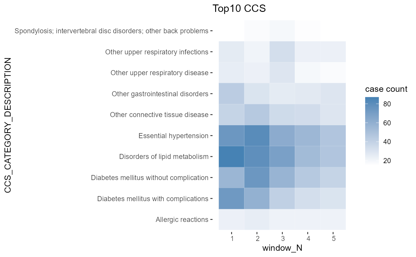
Hazard ratio視覺化
將生存分析後的hazard ratio進行視覺化。
DataFile為從analWindow_Cox的輸出可獲得,pvalue為使用者設定。
head(coxmodel$summarytable[[3]])
#>    features exp(coef) lower .95 upper .95 Pr(>|z|) caseCount
#> 1:  ccs_134     0.482     0.108     2.153    0.339        22
#> 2:  ccs_136         0         0       Inf    0.999         9
#> 3:  ccs_138     2.687     0.276    26.172    0.395        12
#> 4:  ccs_159         0         0       Inf    0.999         8
#> 5:  ccs_197         0         0       Inf    0.999        13
#> 6:  ccs_205     0.873     0.099     7.725    0.903        18
#>                                           CCS_CATEGORY_DESCRIPTION
#> 1:                                 Other upper respiratory disease
#> 2:                                      Disorders of teeth and jaw
#> 3:                                            Esophageal disorders
#> 4:                                        Urinary tract infections
#> 5:                         Skin and subcutaneous tissue infections
#> 6: Spondylosis; intervertebral disc disorders; other back problems
#>                                                    CCS_LVL_2_LABEL
#> 1:                                 Other upper respiratory disease
#> 2:                                      Disorders of teeth and jaw
#> 3:                                Upper gastrointestinal disorders
#> 4:                                  Diseases of the urinary system
#> 5:                         Skin and subcutaneous tissue infections
#> 6: Spondylosis; intervertebral disc disorders; other back problems
#>                                                 CCS_LVL_1_LABEL
#> 1:                           Diseases of the respiratory system
#> 2:                             Diseases of the digestive system
#> 3:                             Diseases of the digestive system
#> 4:                         Diseases of the genitourinary system
#> 5:                 Diseases of the skin and subcutaneous tissue
#> 6: Diseases of the musculoskeletal system and connective tissue
plotHR(DataFile = coxmodel$summarytable[[3]],
       pvalue = 0.05)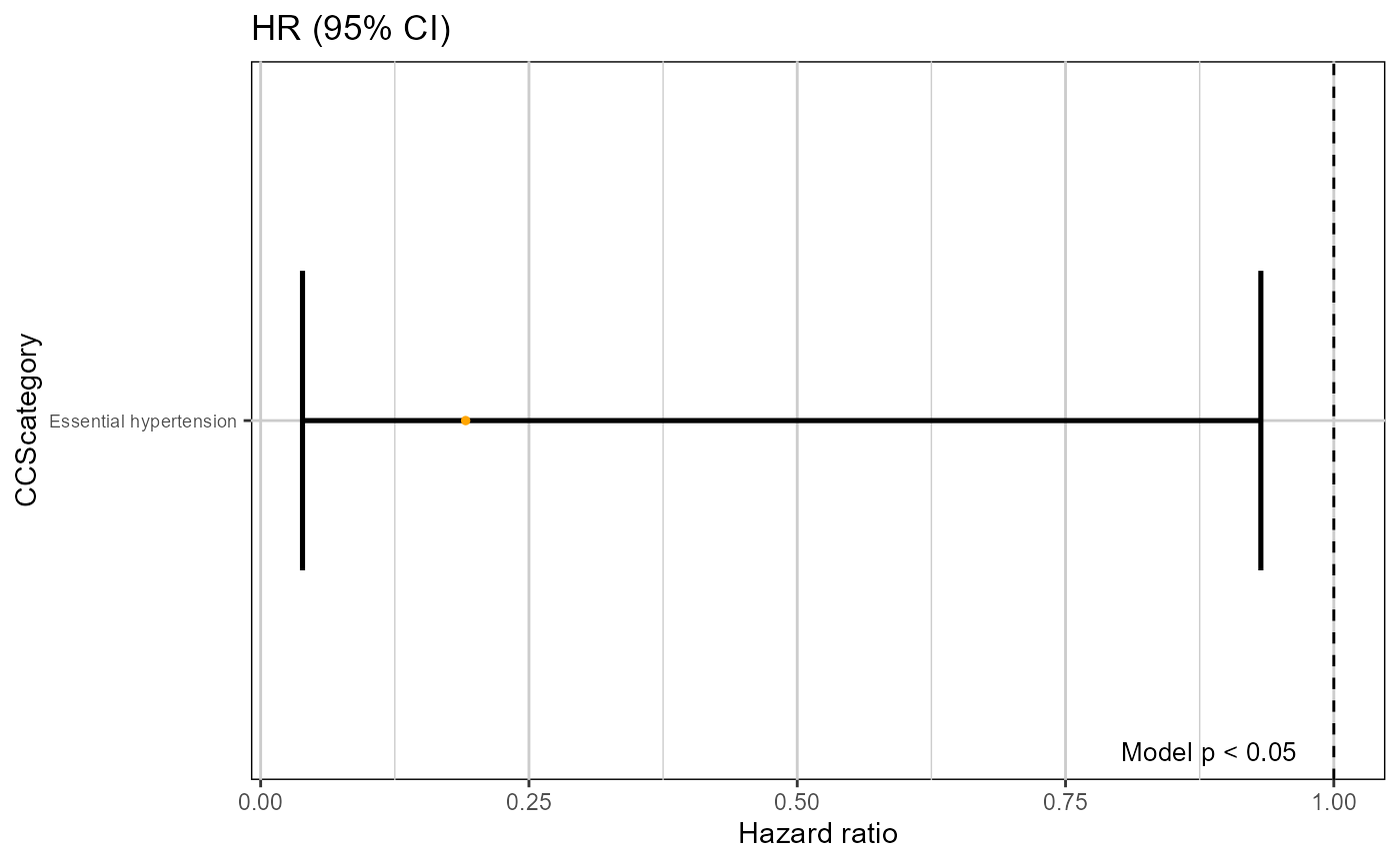
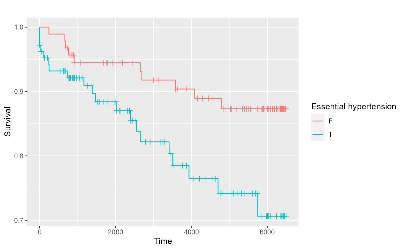
生存區線視覺化
可輸出單個類別變數的存活差異,將病例組與對照組的生存曲線進行視覺化。
var中填入使用者要看的ccs category。
plotSurv(DataFile_cutData = windowcut[window_N=="all"],
         DataFile_personal = personal,
         idColName = ID,
         labelColName = label,
         dataLengthColName = dataLength,
         ccsDescription = "Essential hypertension")
#> Scale for 'colour' is already present. Adding another scale for 'colour',
#> which will replace the existing scale.