Getting started with dxpr: Diagnosis

Description

The proposed open-source dxpr package is a software tool aimed at expediting an integrated analysis of electronic health records (EHRs). By implementing dxpr package, it is easier to integrate, analyze, and visualize clinical data.

In this part, the instruction of how dxpr package works with diagnosis records is provided.

Development version

install.packages("remotes")
# Install development version from GitHub
remotes::install_github("DHLab-TSENG/dxpr")
library(dxpr)

Data Format

dxpr (diagnosis part) is used to pre-process diagnosis codes of EHRs. To execute functions in dxpr, the EHR data input should be a data frame object in R, and contain at least three columns: patient ID, ICD diagnosis codes and date.

Column names or column order of these three columns does not need to necessarily follow a rule. Each required column name will be an argument in functions. Detailed information of required data type of every column and argument of functions can be found in the reference section.

Also, in the R ecosystem, DBI, odbc, and other packages provide access to databases within R. As long as the data is retrieved from databases to a data frame in R, the processes are the same as the following example.

con <- DBI::dbConnect(odbc::odbc(),
                      Driver   = "[your driver's name]",
                      Server   = "[your server's path]",
                      Database = "[your database's name]",
                      UID      = "[Database user]",
                      PWD      = "[Database password]")
dxDataFile <- dbSendQuery(con, "SELECT * FROM example_table WHERE ID = 'sampleID'")
dbFetch(dxDataFile)

Sample file

A sample rda file is included in dxpr package:
This dataset is a simulated medical dataset of 38 patients with overall 300 records.

head(sampleDxFile)
#>     ID  ICD       Date Version
#> 1:  A2 Z992 2020-05-22      10
#> 2:  A5 Z992 2020-01-24      10
#> 3:  A8 Z992 2015-10-27      10
#> 4: A13 Z992 2020-04-26      10
#> 5: A13 Z992 2025-02-02      10
#> 6: A15 Z992 2023-05-12      10

ICD-CM code with two format

dxpr package uses ICD-CM codes as diagnosis standard. There are two formats of ICD-9 and ICD-10 diagnostic codes, decimal (with a decimal point separating the code) and short format, respectively. So two tables of ICD-9-CM and ICD-10-CM are generated to deal with different user needs: ICD9DxwithTwoFormat and ICD10DxwithTwoFormat.

ICD-9-CM

# ICD-9-CM_Short
head(ICD9DxwithTwoFormat$Short)
#> [1] "E0000" "E0001" "E0002" "E0008" "E0009" "E0010"
# ICD-9-CM_Decimal
head(ICD9DxwithTwoFormat$Decimal)
#> [1] "E000.0" "E000.1" "E000.2" "E000.8" "E000.9" "E001.0"

ICD-10-CM

# ICD-10-CM_Short
head(ICD10DxwithTwoFormat$Short)
#> [1] "A000"  "A001"  "A009"  "A0100" "A0101" "A0102"
# ICD-10-CM_Decimal
head(ICD10DxwithTwoFormat$Decimal)
#> [1] "A00.0"  "A00.1"  "A00.9"  "A01.00" "A01.01" "A01.02"

I.Code Integration

A. ICD diagnostic code format transformation：Short <-> Decimal

dxpr package helps users to standardize the ICD-9 and ICD-10 diagnostic codes into a uniform format before further code grouping. The formats used for different grouping methods are shown as Table 1.

Table 1 Format of code classification methods

	ICD format
Clinical Classifications Software (CCS)	short format
Comorbidity	short format
Phenome-Wide Association Studies (PheWAS)	decimal format

Since formats of ICD codes used within a dataset could be different, users can choose a target type (short or decimal) according to the corresponding grouping method.

For example, if a user wants to group data by CCS, then ICD codes should be transformed into short format.

Code standardization for ICD-9 and ICD-10 are executed seperately. There are two ways to distinguish the version of ICD diagnostic code (ICD-9/ICD-10) used in data: one is a specific extra column that records version used (data type in this column should be numeric 9 or 10), the other is a specific date that is the starting date of using ICD-10 in the dataset. For example, reimbursement claims with a date required to use ICD-10 codes in the United States and Taiwan are October 1st, 2015 and January 1st, 2016, respectively.

Warning message

Besides, code standardization functions generate data of diagnosis codes with potential error to help researchers identify the potential coding mistake that may affect the result of following clinical data analysis.

There are two error type：wrong format and wrong version. The former one means the ICD code does not exist (maybe because ICD is wrongly coded or with a wrong place of decimal point). And the latter one means the version is wrong (still use ICD 9 after icd10usingDate, etc.).

Users can check data after receiving the warning message.

dxpr package also provides an overview of error ICD data by Pareto chart (function plotICDError).

A-1. Uniform decimal format

The standardization function icdDxShortToDecimal converts the ICD diagnostic codes to a uniform decimal format, which can be used for grouping diagnostic code to PheWAS classification.

# Short to decimal
decimal <- icdDxShortToDecimal(dxDataFile = sampleDxFile,
                               icdColName = ICD, 
                               dateColName = Date,
                               icd10usingDate = "2015/10/01")
#> Wrong ICD format: total 9 ICD codes (the number of occurrences is in brackets)
#> c("A0.11 (20)", "E114 (8)", "Z9.90 (6)", "F42 (6)", "001 (5)", "75.52 (4)", "755.2 (3)", "123.45 (3)", "7552 (2)")
#>  
#> Wrong ICD version: total 7 ICD codes (the number of occurrences is in brackets)
#> c("V27.0 (18)", "A01.05 (8)", "42761 (7)", "V24.1 (6)", "A0105 (5)", "E03.0 (4)", "650 (4)")
#>  
#> Warning: The ICD mentioned above matches to "NA" due to the format or other
#> issues.
#> Warning: "Wrong ICD format" means the ICD has wrong format
#> Warning: "Wrong ICD version" means the ICD classify to wrong ICD version (cause
#> the "icd10usingDate" or other issues)

In this example, the starting using date of ICD-10 is “2015/10/01” (format: “YYYY/MM/DD”).

Also, there are 9 ICD codes labeled as “wrong format”, and 7 ICD labeled as “wrong version”.

The results are:

decimal$ICD[6:10]
#>       ICD
#> 1:  Z99.2
#> 2:  585.5
#> 3: V45.11
#> 4:  V56.0
#> 5:  585.3

decimal$Error
#>        ICD count IcdVersionInFile     WrongType Suggestion
#>  1:  A0.11    20           ICD 10  Wrong format           
#>  2:  V27.0    18           ICD 10 Wrong version           
#>  3:   E114     8           ICD 10  Wrong format           
#>  4: A01.05     8            ICD 9 Wrong version           
#>  5:  42761     7           ICD 10 Wrong version           
#>  6:  Z9.90     6           ICD 10  Wrong format           
#>  7:    F42     6           ICD 10  Wrong format           
#>  8:  V24.1     6           ICD 10 Wrong version           
#>  9:  A0105     5            ICD 9 Wrong version           
#> 10:    001     5            ICD 9  Wrong format       0019
#> 11:  75.52     4            ICD 9  Wrong format           
#> 12:  E03.0     4            ICD 9 Wrong version           
#> 13:    650     4           ICD 10 Wrong version           
#> 14: 123.45     3           ICD 10  Wrong format           
#> 15:  755.2     3            ICD 9  Wrong format     755.29
#> 16:   7552     2            ICD 9  Wrong format      75529

decimal$Error shows individual error ICD codes in descending order.

A-2. Uniform short format

icdDxDecimalToShort function converts the diagnostic codes to the short format, which can be used for grouping to CCS and comorbidities classification.

# Decimal to short
short <- icdDxDecimalToShort(dxDataFile = sampleDxFile,
                            icdColName = ICD,         
                            dateColName = Date,
                            icd10usingDate = "2015/10/01")
short$ICD[6:10]
#>      ICD
#> 1:  Z992
#> 2:  5855
#> 3: V4511
#> 4:  V560
#> 5:  5853

B. Data integration

Functions in data integration section collapse ICD codes into a smaller number of clinically meaningful categories that are more useful for presenting descriptive statistics than individual ICD diagnostic codes are.

dxpr package supports four strategies to group EHR diagnosis codes, including CCS, PheWAS, comorbidities, and customized defined grouping methods.

The output of code classification contains two data frames.

1) groupedDT

Table 2 groupedDT

Short/Decimal	ID	ICD	Date	GroupType
ICD short/Decimal	patient ID	ICD	Admission date	group of code classification

The original row order of the data is remained the same in groupedDT, and only one extra column GroupType is added.

2) summarised_groupedDT

Table 3 summarised_groupedDT

ID	GroupType	FirstCaseDate	EndCaseDate	Count	Period
patient ID	group of code classification	first admission date	last admission date	counts of period	record period

summarised_groupedDT summarised the ICD codes in the same group of the same patient together.

The two outputs can be used in the following functions. groupedDT can be used to select relevant cases (function selectCases) and calculate condition era (function getConditionEra). summarised_groupedDT can be used to convert the long format of grouped data into a wide format (function groupedDataLongToWide) which is fit to other analytical and plotting packages.

Users can choose the column information of groupType is “category” or “description” (isDescription = TRUE or FALSE)

For example, the ccs description is “Tuberculosis” while the category is “1”.

B-1-1. Clinical Classifications Software (CCS)

The CCS classification for ICD-9 and ICD-10 codes is a diagnostic categorization scheme that can employ in many types of projects analyzing data on diagnoses.

Stop updating since 2019.

1) single-level: icdDxToCCS

Both ICD-9-CM and ICD-10-CM code contains 260 single-level CCS categories which can be corresponded with each other.

## ICD to CCS with category description 
CCS_description <- icdDxToCCS(dxDataFile = sampleDxFile,
                              idColName = ID,
                              icdColName = ICD,        
                              dateColName = Date,
                              icd10usingDate = "2015-10-01",
                              isDescription = TRUE)
head(CCS_description$groupedDT, 5)
#>    Short  ID  ICD       Date CCS_CATEGORY_DESCRIPTION
#> 1:  Z992  A2 Z992 2020-05-22   Chronic kidney disease
#> 2:  Z992  A5 Z992 2020-01-24   Chronic kidney disease
#> 3:  Z992  A8 Z992 2015-10-27   Chronic kidney disease
#> 4:  Z992 A13 Z992 2020-04-26   Chronic kidney disease
#> 5:  Z992 A13 Z992 2025-02-02   Chronic kidney disease
head(CCS_description$summarised_groupedDT, 5)
#>     ID CCS_CATEGORY_DESCRIPTION firstCaseDate endCaseDate count    period
#> 1:  A0   Chronic kidney disease    2009-07-25  2013-12-20     5 1609 days
#> 2:  A1   Chronic kidney disease    2006-11-29  2014-09-24     5 2856 days
#> 3: A10   Chronic kidney disease    2007-11-04  2012-07-30     5 1730 days
#> 4: A11   Chronic kidney disease    2008-03-09  2011-09-03     5 1273 days
#> 5: A12   Chronic kidney disease    2006-05-14  2015-06-29     5 3333 days

## ICD to CCS with category
CCS_category <- icdDxToCCS(dxDataFile = sampleDxFile, 
                          idColName = ID,         
                          icdColName = ICD,       
                          dateColName = Date, 
                          icd10usingDate = "2015-10-01",
                          isDescription = FALSE)
head(CCS_category$groupedDT, 5)
#>    Short  ID  ICD       Date CCS_CATEGORY
#> 1:  Z992  A2 Z992 2020-05-22          158
#> 2:  Z992  A5 Z992 2020-01-24          158
#> 3:  Z992  A8 Z992 2015-10-27          158
#> 4:  Z992 A13 Z992 2020-04-26          158
#> 5:  Z992 A13 Z992 2025-02-02          158
head(CCS_category$summarised_groupedDT, 5)
#>     ID CCS_CATEGORY firstCaseDate endCaseDate count    period
#> 1:  A0          158    2009-07-25  2013-12-20     5 1609 days
#> 2:  A1          158    2006-11-29  2014-09-24     5 2856 days
#> 3: A10          158    2007-11-04  2012-07-30     5 1730 days
#> 4: A11          158    2008-03-09  2011-09-03     5 1273 days
#> 5: A12          158    2006-05-14  2015-06-29     5 3333 days

2) multi-level: icdDxToCCSLvl

Multi-level CCS in ICD-9-CM has four levels, and multi-level CCS in ICD-10-CM has two levels.

## ICD to CCS multiple level 2 description
CCSlvl_description <- icdDxToCCSLvl(dxDataFile = sampleDxFile,
                                    idColName = ID,  
                                    icdColName = ICD,   
                                    dateColName = Date,
                                    icd10usingDate = "2015-10-01",
                                    CCSLevel = 2,
                                    isDescription = TRUE)
head(CCSlvl_description$groupedDT, 5)
#>    Short  ID  ICD       Date                CCS_LVL_2_LABEL
#> 1:  Z992  A2 Z992 2020-05-22 Diseases of the urinary system
#> 2:  Z992  A5 Z992 2020-01-24 Diseases of the urinary system
#> 3:  Z992  A8 Z992 2015-10-27 Diseases of the urinary system
#> 4:  Z992 A13 Z992 2020-04-26 Diseases of the urinary system
#> 5:  Z992 A13 Z992 2025-02-02 Diseases of the urinary system
head(CCSlvl_description$summarised_groupedDT, 5)
#>     ID                CCS_LVL_2_LABEL firstCaseDate endCaseDate count    period
#> 1:  A0 Diseases of the urinary system    2009-07-25  2013-12-20     5 1609 days
#> 2:  A1 Diseases of the urinary system    2006-11-29  2014-09-24     5 2856 days
#> 3: A10 Diseases of the urinary system    2007-11-04  2012-07-30     5 1730 days
#> 4: A11 Diseases of the urinary system    2008-03-09  2011-09-03     5 1273 days
#> 5: A12 Diseases of the urinary system    2006-05-14  2015-06-29     5 3333 days

## ICD to CCS multiple level 3 category
CCSLvl_category <- icdDxToCCSLvl(dxDataFile = sampleDxFile,
                                    idColName = ID,  
                                    icdColName = ICD,   
                                    dateColName = Date,
                                    icd10usingDate = "2015-10-01",
                                    CCSLevel = 3,
                                    isDescription = FALSE)

B-1-2. Clinical Classifications Software Refined (CCSR)

The CCSR classification for ICD-10 codes is a diagnostic categorization scheme that can employ in many types of projects analyzing data on diagnoses.

Unlike CCS, a diagnosis code can be classified into more than one categories in CCSR. However, it is only applicable to ICD-10.

## ICD to CCSR with category description 
CCSR_description <- icdDxToCCSR(dxDataFile = sampleDxFile,
                              idColName = ID,
                              icdColName = ICD,        
                              dateColName = Date,
                              icd10usingDate = "2015-10-01",
                              isDescription = TRUE)
head(CCSR_description$groupedDT, 5)
#>    Short  ID  ICD       Date CCSR_CATEGORY_DESCRIPTION
#> 1:  Z992  A2 Z992 2020-05-22    Other specified status
#> 2:  Z992  A5 Z992 2020-01-24    Other specified status
#> 3:  Z992  A8 Z992 2015-10-27    Other specified status
#> 4:  Z992 A13 Z992 2020-04-26    Other specified status
#> 5:  Z992 A13 Z992 2025-02-02    Other specified status
head(CCSR_description$summarised_groupedDT, 5)
#>     ID CCSR_CATEGORY_DESCRIPTION firstCaseDate endCaseDate count    period
#> 1: A13    Other specified status    2020-04-26  2025-02-02     2 1743 days
#> 2: A15    Other specified status    2023-05-12  2023-05-12     1    0 days
#> 3:  A2    Other specified status    2020-05-22  2020-05-22     1    0 days
#> 4:  A5    Other specified status    2020-01-24  2020-01-24     1    0 days
#> 5:  A8    Other specified status    2015-10-27  2015-10-27     1    0 days

B-2. PheWAS

The dxpr package applied PheWAS, performing a hierarchical grouping of ICD-9 diagnostic codes and ICD-10 diagnostic codes (beta version).

## ICD to PheWAS
PheWAS <- icdDxToPheWAS(dxDataFile = sampleDxFile,
                         idColName = ID,           
                         icdColName = ICD,     
                         dateColName = Date,
                         icd10usingDate = "2015-10-01",
                         isDescription = FALSE)
PheWAS$groupedDT[7:11]
#>    Decimal ID   ICD       Date PheCode
#> 1:   585.5 A0  5855 2013-12-20  585.32
#> 2:  V45.11 A0 V4511 2012-04-05  585.31
#> 3:   V56.0 A0  V560 2010-03-28  585.31
#> 4:   585.3 A0  5853 2010-10-29  585.33
#> 5:   585.6 A0  5856 2009-07-25  585.32
PheWAS$summarised_groupedDT[7:11]
#>    ID PheCode firstCaseDate endCaseDate count    period
#> 1: A0  585.31    2010-03-28  2012-04-05     2  739 days
#> 2: A0  585.33    2010-10-29  2010-10-29     1    0 days
#> 3: A1  585.32    2006-11-29  2013-04-28     3 2342 days
#> 4: A1  585.33    2014-09-24  2014-09-24     1    0 days
#> 5: A1  585.31    2008-06-25  2008-06-25     1    0 days

B-3. Comorbidities

The dxpr package provides three grouping methods of comorbidity as below:

1) AHRQ

AHRQ comorbidity measure dataset is based on AHRQ Elixhauser Comorbidity Index.

AHRQ <- icdDxToComorbid(dxDataFile = sampleDxFile,
                        idColName = ID,           
                        icdColName = ICD,       
                        dateColName = Date,
                        icd10usingDate = "2015-10-01",
                        comorbidMethod = AHRQ)
AHRQ$groupedDT[160:164]
#>     Short ID    ICD       Date Comorbidity
#> 1: M06821 D1 M06821 2016-12-06   Rheumatic
#> 2:  K7291 D1  K7291 2024-04-04       Liver
#> 3: O99353 D2 O99353 2023-10-23  NeuroOther
#> 4: F13230 D2 F13230 2022-09-15       Drugs
#> 5:  C8397 D2  C8397 2019-10-13    Lymphoma
head(AHRQ$summarised_groupedDT, 5)
#>     ID Comorbidity firstCaseDate endCaseDate count    period
#> 1:  A0       Renal    2009-07-25  2013-12-20     5 1609 days
#> 2:  A1       Renal    2006-11-29  2014-09-24     5 2856 days
#> 3: A10       Renal    2007-11-04  2012-07-30     5 1730 days
#> 4: A11       Renal    2008-03-09  2011-09-03     5 1273 days
#> 5: A12       Renal    2006-05-14  2015-06-29     5 3333 days

2) Charlson

Charlson comorbidity measure dataset is based on Quan’s translations of the Charlson Comorbidity Index.

Charlson <- icdDxToComorbid(dxDataFile = sampleDxFile,
                        idColName = ID,           
                        icdColName = ICD,       
                        dateColName = Date,
                        icd10usingDate = "2015-10-01",
                        comorbidMethod = charlson)
Charlson$groupedDT[160:164]
#>     Short ID    ICD       Date Comorbidity
#> 1: M06821 D1 M06821 2016-12-06       Rheum
#> 2:  K7291 D1  K7291 2024-04-04        MSLD
#> 3: O99353 D2 O99353 2023-10-23        <NA>
#> 4: F13230 D2 F13230 2022-09-15        <NA>
#> 5:  C8397 D2  C8397 2019-10-13      CANCER
head(Charlson$summarised_groupedDT, 5)
#>     ID Comorbidity firstCaseDate endCaseDate count    period
#> 1:  A0          RD    2009-07-25  2013-12-20     5 1609 days
#> 2:  A1          RD    2006-11-29  2014-09-24     5 2856 days
#> 3: A10          RD    2007-11-04  2012-07-30     5 1730 days
#> 4: A11          RD    2008-03-09  2011-09-03     5 1273 days
#> 5: A11      DIAB_C    2015-12-16  2015-12-16     1    0 days

3) Elixhauser

The Elixhauser comorbidity software is one in a family of databases and software tools developed as part of the Healthcare Cost and Utilization Project (HCUP).

ELIX <- icdDxToComorbid(dxDataFile = sampleDxFile,
                        idColName = ID,           
                        icdColName = ICD,       
                        dateColName = Date,
                        icd10usingDate = "2015-10-01",
                        comorbidMethod = elix)
ELIX$groupedDT[160:164]
#>     Short ID    ICD       Date Comorbidity
#> 1: M06821 D1 M06821 2016-12-06        ARTH
#> 2:  K7291 D1  K7291 2024-04-04       LIVER
#> 3: O99353 D2 O99353 2023-10-23       NEURO
#> 4: F13230 D2 F13230 2022-09-15        DRUG
#> 5:  C8397 D2  C8397 2019-10-13       LYMPH
head(ELIX$summarised_groupedDT, 5)
#>     ID Comorbidity firstCaseDate endCaseDate count    period
#> 1:  A0    RENLFAIL    2009-07-25  2013-12-20     5 1609 days
#> 2:  A1    RENLFAIL    2006-11-29  2014-09-24     5 2856 days
#> 3: A10    RENLFAIL    2007-11-04  2012-07-30     5 1730 days
#> 4: A11    RENLFAIL    2008-03-09  2011-09-03     5 1273 days
#> 5: A12    RENLFAIL    2006-05-14  2015-06-29     5 3333 days

B-4. Customize group method

The dxpr package provided customized grouping functions, in which researches can define the grouping categories; therefore, it is more flexible for grouping ICD diagnostic codes.

For example, researcher can declare a customized grouping table for chronic kidney disease category, and convert an existing dataset into a grouped chronic kidney disease dataset.

There are two functions for customized defined grouping method based on precise and fuzzy grouping method, respectively.

1) Precise method: icdDxToCustom

# CustomGroupingTable 
groupingTable <- data.frame(Group = rep("Chronic kidney disease",6),
                            ICD = c("N181","5853","5854","5855","5856","5859"),
                            stringsAsFactors = FALSE)
CustomGroup <- icdDxToCustom(dxDataFile = sampleDxFile,  
                             idColName = ID,         
                             icdColName = ICD,  
                             dateColName = Date,
                             customGroupingTable = groupingTable)
CustomGroup$groupedDT[10:14]
#>     ICD ID       Date                  Group
#> 1: 5853 A0 2010-10-29 Chronic kidney disease
#> 2: 5856 A0 2009-07-25 Chronic kidney disease
#> 3: 5856 A1 2006-11-29 Chronic kidney disease
#> 4: 5855 A1 2012-06-19 Chronic kidney disease
#> 5: 5855 A1 2013-04-28 Chronic kidney disease
head(CustomGroup$summarised_groupedDT, 5)
#>     ID                  Group firstCaseDate endCaseDate count    period
#> 1:  A0 Chronic kidney disease    2009-07-25  2013-12-20     3 1609 days
#> 2:  A1 Chronic kidney disease    2006-11-29  2014-09-24     4 2856 days
#> 3: A10 Chronic kidney disease    2007-11-04  2007-11-04     1    0 days
#> 4: A11 Chronic kidney disease    2008-03-09  2010-02-21     2  714 days
#> 5: A12 Chronic kidney disease    2006-05-14  2011-02-25     3 1748 days

2) Fuzzy method: icdDxToCustomGrep

# CustomGroupingTable
grepTable <- data.frame(Group = "Chronic kidney disease",
                        grepIcd = "^585|^N18",
                        stringsAsFactors = FALSE)
CustomGrepGroup <- icdDxToCustomGrep(dxDataFile = sampleDxFile, 
                                    idColName = ID,            
                                    icdColName = ICD,   
                                    dateColName = Date,
                                    customGroupingTable = grepTable)
CustomGrepGroup$groupedDT[10:14]
#>    ID  ICD       Date            GrepedGroup
#> 1: A0 5853 2010-10-29 Chronic kidney disease
#> 2: A0 5856 2009-07-25 Chronic kidney disease
#> 3: A1 5856 2006-11-29 Chronic kidney disease
#> 4: A1 5855 2012-06-19 Chronic kidney disease
#> 5: A1 5855 2013-04-28 Chronic kidney disease
head(CustomGrepGroup$summarised_groupedDT, 5)
#>     ID            GrepedGroup firstCaseDate endCaseDate count    period
#> 1:  A0 Chronic kidney disease    2009-07-25  2013-12-20     3 1609 days
#> 2:  A1 Chronic kidney disease    2006-11-29  2014-09-24     4 2856 days
#> 3: A10 Chronic kidney disease    2007-11-04  2007-11-04     1    0 days
#> 4: A11 Chronic kidney disease    2008-03-09  2010-02-21     2  714 days
#> 5: A12 Chronic kidney disease    2006-05-14  2011-02-25     3 1748 days

II. Data Wrangling

A. Cases selection

The query function selectCases can select the cases matching defined case conditions (been diagnosed with certain condition for certain times within a specific duration). User can select cases by diagnostic categories, such as CCS category, ICD codes, etc.

The output of this function provides the start and end dates of the cases, the number of days between them, and the most common ICD codes used in the case definition. 　　　

Case <- selectCases(dxDataFile = sampleDxFile,
                    idColName = ID,           
                    icdColName = ICD,       
                    dateColName = Date,
                    groupDataType = ccslvl2,
                    icd10usingDate = "2015/10/01",
                    caseCondition = "Diseases of the urinary system",
                    caseCount = 1,
                    caseName = "Selected")
head(Case)                   
#>     ID selectedCase count firstCaseDate endCaseDate    period MostCommonICD
#> 1:  A3     Selected     5    2008-07-08  2014-02-24 2057 days          V420
#> 2:  A1     Selected     5    2006-11-29  2014-09-24 2856 days          5855
#> 3: A10     Selected     5    2007-11-04  2012-07-30 1730 days         V5631
#> 4: A12     Selected     5    2006-05-14  2015-06-29 3333 days          5859
#> 5: A13     Selected     5    2006-04-29  2025-02-02 6854 days          5855
#> 6: A15     Selected     5    2007-05-25  2023-05-12 5831 days         V5631
#>    MostCommonICDCount
#> 1:                  3
#> 2:                  2
#> 3:                  2
#> 4:                  2
#> 5:                  2
#> 6:                  2

B. Get eligible period of patient records

The function getEligiblePeriod is used for querying the earliest and latest admission date for each patient.

admissionDate <- getEligiblePeriod(dxDataFile = sampleDxFile,
                                   idColName = ID,
                                   dateColName = Date)
head(admissionDate)                                  
#>     ID firstRecordDate endRecordDate
#> 1:  D6      2005-10-09    2025-01-05
#> 2: A12      2006-01-12    2022-06-12
#> 3:  D1      2006-02-12    2024-04-04
#> 4: A13      2006-04-29    2025-02-02
#> 5:  A9      2006-06-30    2023-12-10
#> 6:  D2      2006-09-01    2025-08-11

C. Data split

Function splitDataByDate extracts data by a specific clinical event (e.g., first diagnosis dates of chronic diseases).
Users can define a table of clinical index dates of each patient. The date can generate by selectCases function or first/last admission date by getEligiblePeriod function.

This function can split data through classifying the data recorded before or after the defined index date and calculating the period between the record date and index date based on a self-defined window gap.

indexDateTable <- data.frame(ID = c("A0","B0","C0","D0"),
                             indexDate = c("2009-07-25", "2015-12-26",
                                           "2015-12-05", "2017-01-29"),
                             stringsAsFactors = FALSE)

Data <- splitDataByDate(dxDataFile = sampleDxFile,
                        idColName = ID,
                        icdColName = ICD,
                        dateColName = Date,
                        indexDateFile = indexDateTable,
                        gap = 30) 
head(Data, 5)
#>    ID   ICD       Date  indexDate timeTag window
#> 1: A0  5856 2009-07-25 2009-07-25       A      1
#> 2: A0  V560 2010-03-28 2009-07-25       A      9
#> 3: A0  5853 2010-10-29 2009-07-25       A     16
#> 4: A0 V4511 2012-04-05 2009-07-25       A     33
#> 5: A0  5855 2013-12-20 2009-07-25       A     54

D. Condition era

The concept of condition era is committed to the length of the persistence gap: when the time interval of any two consecutive admissions for certain conditions is smaller than the length of the persistence gap, then these two admission events will be aggregated into the same condition era.

Function getConditionEra calculates condition era by using the grouped categories or self-defining groups of each patient and then generates a table with individual IDs, the first and last record of an era, and the sequence number of each episode.

Era <- getConditionEra(dxDataFile = sampleDxFile,
                       idColName = ID,
                       icdColName = ICD,
                       dateColName = Date,
                       icd10usingDate = "2015-10-01", 
                       gapDate = 30,
                       groupDataType = ccs,
                       isDescription = FALSE)
head(Era)                       
#>    ID CCS_CATEGORY era firstCaseDate endCaseDate count period
#> 1: A0          158   1    2009-07-25  2009-07-25     1 0 days
#> 2: A0          158   2    2010-03-28  2010-03-28     1 0 days
#> 3: A0          158   3    2010-10-29  2010-10-29     1 0 days
#> 4: A0          158   4    2012-04-05  2012-04-05     1 0 days
#> 5: A0          158   5    2013-12-20  2013-12-20     1 0 days
#> 6: A1          158   1    2006-11-29  2006-11-29     1 0 days

E. EDA preparation

After data integration, dxpr package provides a function to convert long format of grouped data into wide format which is fit to other analytical and plotting packages.

There are two type of output: numeric and binary (numericOrBinary = B or N )

#binary
groupedData_Wide <- groupedDataLongToWide(dxDataFile = ELIX$groupedDT, 
                                          idColName = ID,    
                                          categoryColName = Comorbidity,   
                                          dateColName = Date,
                                          numericOrBinary = B)
                                          
head(groupedData_Wide, 5)
#>     ID  ARTH CHRNLUNG  DMCX  DRUG HRENWORF HTNPREG LIVER LYMPH NEURO OBESE
#> 1:  A0 FALSE    FALSE FALSE FALSE    FALSE   FALSE FALSE FALSE FALSE FALSE
#> 2:  A1 FALSE    FALSE FALSE FALSE    FALSE   FALSE FALSE FALSE FALSE FALSE
#> 3: A10 FALSE    FALSE FALSE FALSE    FALSE   FALSE FALSE FALSE FALSE FALSE
#> 4: A11 FALSE    FALSE FALSE FALSE    FALSE   FALSE FALSE FALSE FALSE FALSE
#> 5: A12 FALSE    FALSE FALSE FALSE    FALSE   FALSE FALSE FALSE FALSE FALSE
#>     PARA PERIVASC PSYCH RENLFAIL TUMOR ULCER VALVE WGHTLOSS
#> 1: FALSE    FALSE FALSE     TRUE FALSE FALSE FALSE    FALSE
#> 2: FALSE    FALSE FALSE     TRUE FALSE FALSE FALSE    FALSE
#> 3: FALSE    FALSE FALSE     TRUE FALSE FALSE FALSE    FALSE
#> 4: FALSE    FALSE FALSE     TRUE FALSE FALSE FALSE    FALSE
#> 5: FALSE    FALSE FALSE     TRUE FALSE FALSE FALSE    FALSE

# numeric
groupedData_Wide <- groupedDataLongToWide(dxDataFile = ELIX$groupedDT, 
                                          idColName = ID,    
                                          categoryColName = Comorbidity,   
                                          dateColName = Date,
                                          numericOrBinary = N)
head(groupedData_Wide, 5)
#>     ID ARTH CHRNLUNG DMCX DRUG HRENWORF HTNPREG LIVER LYMPH NEURO OBESE PARA
#> 1:  A0    0        0    0    0        0       0     0     0     0     0    0
#> 2:  A1    0        0    0    0        0       0     0     0     0     0    0
#> 3: A10    0        0    0    0        0       0     0     0     0     0    0
#> 4: A11    0        0    0    0        0       0     0     0     0     0    0
#> 5: A12    0        0    0    0        0       0     0     0     0     0    0
#>    PERIVASC PSYCH RENLFAIL TUMOR ULCER VALVE WGHTLOSS
#> 1:        0     0        5     0     0     0        0
#> 2:        0     0        5     0     0     0        0
#> 3:        0     0        5     0     0     0        0
#> 4:        0     0        5     0     0     0        0
#> 5:        0     0        5     0     0     0        0

III. Visualization

Visualization provides overview of clinical data.

A. Pareto chart of error ICD list

Through code standardization, the functions icdDxDecimalToShort and icdDxShortToDecimal generate a table of diagnosis codes with potential errors.

The Pareto chart includes bar plot and line chart to visualize individual possible error ICD codes represented in descending order and cumulative total.

error <- icdDxDecimalToShort(dxDataFile = sampleDxFile,
                            icdColName = ICD,
                            dateColName = Date,
                            icd10usingDate = "2015/10/01")
Plot_error1 <- plotICDError(errorFile = error$Error,
                            icdVersion = all,
                            wrongICDType = all,
                            others = TRUE,
                            topN = 10)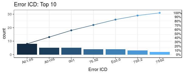

For instance, if a user chooses top 10 of common error ICD in dataset (topN = 10), then the Pareto chart output shows with top 10 error codes in this dataset and a list of the detail of error ICD codes.

Plot_error1$ICD
#>        ICD count CumCountPerc IcdVersionInFile     WrongType Suggestion
#>  1:  A0.11    20       18.35%           ICD 10  Wrong format           
#>  2:  V27.0    18       34.86%           ICD 10 Wrong version           
#>  3:   E114     8        42.2%           ICD 10  Wrong format           
#>  4: A01.05     8       49.54%            ICD 9 Wrong version           
#>  5:  42761     7       55.96%           ICD 10 Wrong version           
#>  6:  Z9.90     6       61.47%           ICD 10  Wrong format           
#>  7:    F42     6       66.97%           ICD 10  Wrong format           
#>  8:  V24.1     6       72.48%           ICD 10 Wrong version           
#>  9:  A0105     5       77.06%            ICD 9 Wrong version           
#> 10:    001     5       81.65%            ICD 9  Wrong format       0019
#> 11: others    20         100%            ICD 9  Wrong format

The most common error ICD is A0.11 which has 20 admission records and error type is “wrong format”

Also, users can divide ICD-9 by the prefix of the ICD code: 0, 1, 2,…, 9, V and E (groupICD = TRUE)

ICD-9-CM divided into 19 chapters:
　001-139: Infectious And Parasitic Diseases
　140-239: Neoplasms
　….

For instance, if user chooses top 3 of common error ICD-9, the output Pareto chart shows with top 3 error codes and a list of the detail of error ICD codes.

Plot_error2 <- plotICDError(errorFile = error$Error,
                             icdVersion = 9,
                             wrongICDType = all,
                             groupICD = TRUE,
                             others = TRUE,
                             topN = 3)
#> Warning: `guides(<scale> = FALSE)` is deprecated. Please use `guides(<scale> =
#> "none")` instead.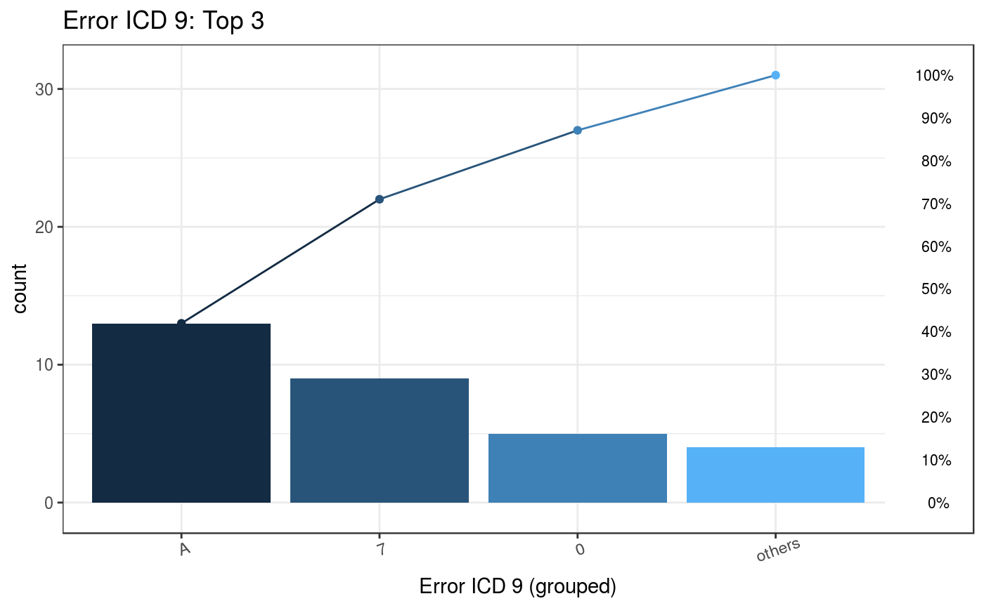

Plot_error2$ICD
#>    ICDGroup groupCount CumCountPerc MostICDInGroup ICDPercInGroup     WrongType
#> 1:        A         13       41.94%         A01.05         61.54% Wrong version
#> 2:        7          9       70.97%          75.52         44.44%  Wrong format
00#> 3:        0          5        87.1%            001           100%  Wrong format
#> 4:   Others          4         100%          E03.0           100% Wrong version

The most common error ICD is A01.05 which has 13 admission records and the error type is “wrong version”.

B. histogram plot

plotDiagCat function provides an overview of grouping category of the diagnostic code in histogram plot. User can observe the proportion of diagnostic categories in their dataset.

groupedDataWide <- groupedDataLongToWide(ELIX$groupedDT,
                                         idColName = ID,
                                         categoryColName = Comorbidity,
                                         dateColName = Date)
plot1 <- plotDiagCat(groupedDataWide = groupedDataWide,
                     idColName = ID,
                     topN = 10,
                     limitFreq = 0.01)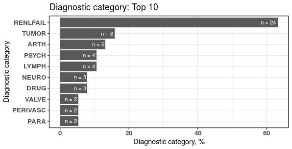

The first group, for instance, is grouped into “RENLFAIL” of ELIX comorbidity index.

plot1$sigCate
#>     DiagnosticCategory  N Percentage
#>  1:           RENLFAIL 24      63.16
#>  2:              TUMOR  6      15.79
#>  3:               ARTH  5      13.16
#>  4:              LYMPH  4      10.53
#>  5:              PSYCH  4      10.53
#>  6:               DRUG  3       7.89
#>  7:              NEURO  3       7.89
#>  8:               PARA  2       5.26
#>  9:           PERIVASC  2       5.26
#> 10:              VALVE  2       5.26

This function can also do the Chi-square test and Fisher’s exact test to see if it is statistical significantly different between the diagnostic categories of case and control. The default level of significance is of 5% (p = 0.05).

selectedCaseFile <- selectCases(dxDataFile = sampleDxFile,
                                idColName = ID,
                                icdColName = ICD,
                                dateColName = Date,
                                icd10usingDate = "2015/10/01",
                                groupDataType = ccslvl2,
                                caseCondition = "Diseases of the urinary system",
                                caseCount = 1)
                                
groupedDataWide <- groupedDataLongToWide(ELIX$groupedDT, ID, Comorbidity, Date,
                                         selectedCaseFile = selectedCaseFile)
plot2 <- plotDiagCat(groupedDataWide = groupedDataWide,
                     idColName = ID,
                     groupColName = selectedCase,
                     topN = 10,
                     limitFreq = 0.01,
                     pvalue = 0.05)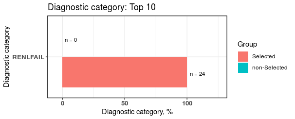

There are stastitcal significant difference in “RENLFAIL” of ELIX comorbidity index between case and control.

plot2$sigCate
#>    DiagnosticCategory        Group  N Percentage
#> 1:           RENLFAIL non-Selected  0          0
#> 2:           RENLFAIL     Selected 24        100