5. NumPy

Yi-Ju Tseng

NumPy

• Basic NumPy
• Universal Functions (UFuncs) in NumPy
• Aggregations
• Broadcasting
• Boolean Arrays and Masks

NumPy

• Basic NumPy
• Universal Functions (UFuncs) in NumPy
• Aggregations
• Broadcasting
• Boolean Arrays and Masks

Basic NumPy

What is NumPy?

• Numerical Python
• Contain values of a single type
• the fundamental package for numerical computation in Python
• high-performance multidimensional array object + tools for working with these arrays
• foundation of other data science libraries (Pandas, SciPy, and scikit-learn)
• Key feature: ndarray n-dimensional array object

Why Use NumPy Arrays?

• Efficiency: more compact than Python lists
• Speed: vectorized operations on NumPy arrays are much faster than iterating through Python lists (optimized C)
• Functionality: provides a large library of mathematical functions

NumPy Getting Started

Install

!pip3 install numpy # ! for shell script

Import

import numpy as np

Create NumPy array (Recap)

Check Ch.3 for more information

• np.full(dim, value): repeated values
• 2d dimension: (row, column)

np.full((2, 4), 3.14)

array([[3.14, 3.14, 3.14, 3.14],
       [3.14, 3.14, 3.14, 3.14]])

• np.random.random(dim)
• np.random.normal(mean,sd,dim)

np.random.random((2,3))

array([[0.51327059, 0.95227437, 0.76479752],
       [0.69856383, 0.22922456, 0.43017838]])

np.random.normal(0,1,(2,3))

array([[-0.20241711,  2.754591  ,  0.0571311 ],
       [ 1.75228413, -0.08813171,  0.12377476]])

Basic NumPy Array Manipulations

• Attributes: Size, shape, memory consumption, and data types of arrays
• Indexing: Getting and setting the value of individual array elements
• Slicing: Getting and setting smaller subarrays within a larger array
• Reshaping: Changing the shape of a given array
• Joining and splitting: Combining multiple arrays into one, and splitting one array into many

NumPy Array Attributes

• Every NumPy array has attributes:
  • ndim: the number of dimensions
  • shape: the size of each dimension
  • size: the total size of the array
  • dtype: the data type of the array elements
  • itemsize: the size (in bytes) of each array element
  • nbytes: the total size (in bytes) of the array

NumPy Array Attributes - Examples

np.random.seed(0)  # seed for reproducibility
x1 = np.random.randint(10, size=6)  # One-dimensional array
x2 = np.random.randint(10, size=(3, 4))  # Two-dimensional array
x3 = np.random.randint(10, size=(3, 4, 5))  # Three-dimensional array

print(x1)
print("ndim: ", x1.ndim)
print("shape:", x1.shape)
print("size: ", x1.size)
print("dtype: ", x1.dtype)
print("itemsize:", x1.itemsize, "bytes")
print("nbytes: ", x1.nbytes, "bytes")

[5 0 3 3 7 9]
ndim:  1
shape: (6,)
size:  6
dtype:  int64
itemsize: 8 bytes
nbytes:  48 bytes

print(x2)
print("ndim: ", x2.ndim)
print("shape:", x2.shape)
print("size: ", x2.size)
print("dtype: ", x2.dtype)
print("itemsize:", x2.itemsize, "bytes")
print("nbytes: ", x2.nbytes, "bytes")

[[3 5 2 4]
 [7 6 8 8]
 [1 6 7 7]]
ndim:  2
shape: (3, 4)
size:  12
dtype:  int64
itemsize: 8 bytes
nbytes:  96 bytes

NumPy Array Attributes - data type

• NumPy arrays contain values of a single type
• dtype: Assign data type when creating a numpy array
  • Most of the time, this can be automatically detected
  • Available data type: ref

np.zeros(10, dtype=np.int16)

array([0, 0, 0, 0, 0, 0, 0, 0, 0, 0], dtype=int16)

Array Indexing - Single Elements

• Similar to lists
• In a multi-dimensional array, items can be accessed using a comma-separated indices
• Indexing starts from 0

Array Indexing - Example

• x[row, column]
• -1: last index

x = np.array([[1,2,3],[4,5,6]])
print(x)

[[1 2 3]
 [4 5 6]]

print(x[0, 0]) 

1

print(x[1, 2])  

6

x[0, 0] = 12
print(x)

[[12  2  3]
 [ 4  5  6]]

x[-1, -1] = 24
print(x)

[[12  2  3]
 [ 4  5 24]]

Array Slicing - Subarrays

• Colon (:) operator: slice arrays
• x[start:stop:step]
• Default:
  • start=0
  • stop=size of dimension
  • step=1

Array Slicing - Example (1D)

x = np.arange(10)
x

array([0, 1, 2, 3, 4, 5, 6, 7, 8, 9])

x[start:stop:step]

print(x[1:5]) # Elements 1 to 4
print(x[:5:2]) # Every other element from beginning to index 5
print(x[::2]) # Every other element from the beginning
print(x[5:]) # Elements starting at index 5

[1 2 3 4]
[0 2 4]
[0 2 4 6 8]
[5 6 7 8 9]

Array Slicing - Example (2D)

two_d = np.array([np.arange(5),np.arange(5,10)]) 
print(two_d)

[[0 1 2 3 4]
 [5 6 7 8 9]]

empty slice (:)

print(two_d[1,:])

[5 6 7 8 9]

print(two_d[:,1])

[1 6]

print(two_d[1,-1])

9

can be omitted in row access

print(two_d[1])

[5 6 7 8 9]

print(two_d[:2])

[[0 1 2 3 4]
 [5 6 7 8 9]]

print(two_d[1][2])

7

No Copy View

• In NumPy array, slices will be View. in lists, slices will be copies
• .copy() if you need a copy

print(x2)

[[3 5 2 4]
 [7 6 8 8]
 [1 6 7 7]]

x2_sub = x2[:2, :2]
print(x2_sub)

[[3 5]
 [7 6]]

x2_sub[0, 0] = 99
print(x2_sub)

[[99  5]
 [ 7  6]]

print(x2)

[[99  5  2  4]
 [ 7  6  8  8]
 [ 1  6  7  7]]

Reshaping of Arrays

• reshape(dim): gives a new shape to an array
• the size must match

x = np.arange(1, 10)
x

array([1, 2, 3, 4, 5, 6, 7, 8, 9])

grid = x.reshape((3, 3))
print(grid)

[[1 2 3]
 [4 5 6]
 [7 8 9]]

Hands-on - Indexing and Slicing - 1

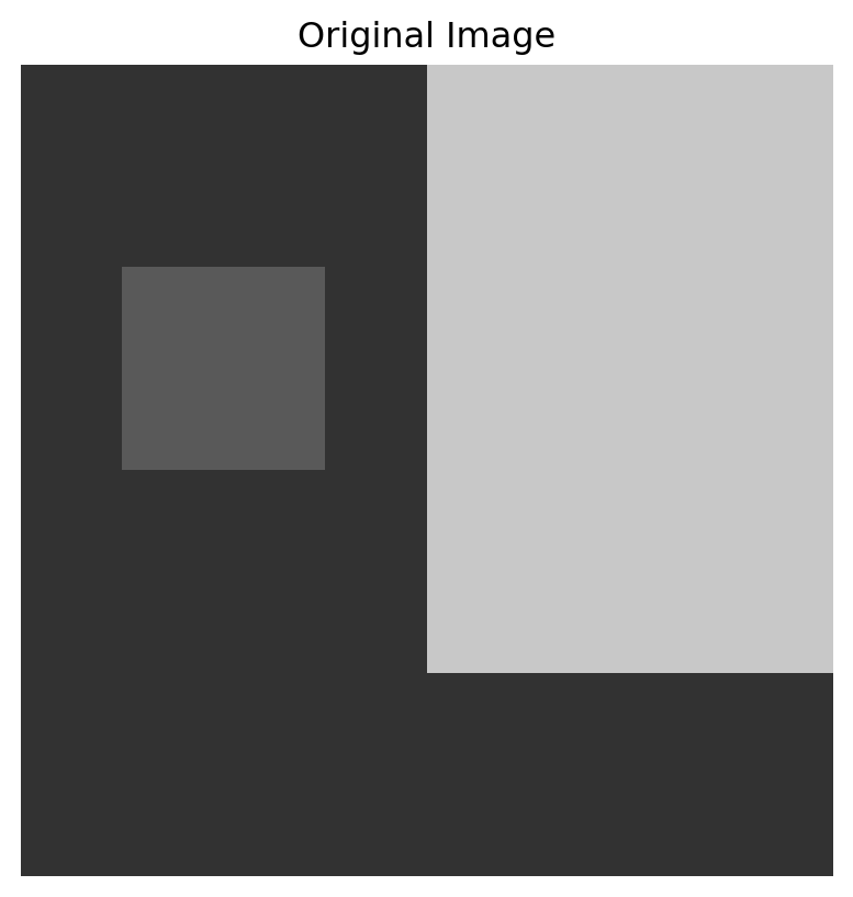
You’re working on a project to analyze and manipulate digital images using NumPy. Your task is to perform various operations on image data represented as NumPy arrays.

import numpy as np
import matplotlib.pyplot as plt
# Create a sample 8x8 grayscale image (0-255 values)
image = np.array([
    [50, 50, 50, 50, 200, 200, 200, 200],
    [50, 50, 50, 50, 200, 200, 200, 200],
    [50, 90, 90, 50, 200, 200, 200, 200],
    [50, 90, 90, 50, 200, 200, 200, 200],
    [50, 50, 50, 50, 200, 200, 200, 200],
    [50, 50, 50, 50, 200, 200, 200, 200],
    [50, 50, 50, 50, 50, 50, 50, 50],
    [50, 50, 50, 50, 50, 50, 50, 50]
])

Hands-on - Indexing and Slicing - 2

# Function to display the image
def show_image(img, title="Image"):
    plt.imshow(img, cmap='gray', vmin=0, vmax=255)
    plt.title(title)
    plt.axis('off')
    plt.show()

show_image(image, "Original Image")

Hands-on - Indexing and Slicing - 3

• Extract the 4x4 sub-image from the top-left corner.
• Extract every other pixel from both dimensions (creating a 4x4 image).
• Flatten the image into a 1D array.
• Reshape the flattened array back into an 8x8 image.

Array Concatenation and Splitting

• np.concatenate([array1, array2, ...]): Concatenates arrays along an existing (or first) axis.
• np.vstack([array1, array2]): Vertical stack (row-wise concatenation).
• np.hstack([array1, array2]): Horizontal stack (column-wise concatenation).

Concatenation - Example

np.concatenate([array1, array2, ...]): Concatenates arrays along an existing (or first) axis.

x = np.array([1, 2, 3])
y = np.array([3, 2, 1])
z = [99, 99, 99]
print(np.concatenate([x, y, z]))

[ 1  2  3  3  2  1 99 99 99]

Concatenation - Example

np.concatenate([array1, array2, ...]): Concatenates arrays along an existing (or first) axis.

grid = np.array([[1, 2, 3],
                 [4, 5, 6]])
np.concatenate([grid, grid])                 

array([[1, 2, 3],
       [4, 5, 6],
       [1, 2, 3],
       [4, 5, 6]])

Set axis=1 for the second axis

np.concatenate([grid, grid], axis=1)                 

array([[1, 2, 3, 1, 2, 3],
       [4, 5, 6, 4, 5, 6]])

Concatenation - np.vstack

• np.vstack([array1, array2]): Vertical stack (row-wise concatenation).

x = np.array([1, 2, 3])
grid = np.array([[9, 8, 7],
                 [6, 5, 4]])
np.vstack([x, grid])           

array([[1, 2, 3],
       [9, 8, 7],
       [6, 5, 4]])

Concatenation - np.hstack

• np.hstack([array1, array2]): Horizontal stack (column-wise concatenation).

y = np.array([[99],
              [99]])
np.hstack([grid, y])       

array([[ 9,  8,  7, 99],
       [ 6,  5,  4, 99]])

Splitting

The opposite of concatenation is splitting

• np.split(np array,[split points]) or np.split(np array, # of sections)
• np.vsplit(np array,[split points]) or np.vsplit(np array, # of sections)
• np.hsplit(np array,[split points]) or np.hsplit(np array, # of sections)
• split points: split before the split point
  • N split-points, leads to N + 1 subarrays
• # of sections: divided into N equal arrays

Splitting

split points

x = np.array([1, 2, 3, 99, 99, 3, 2, 1])
x1, x2, x3 = np.split(x, [3, 5])
print(x1, x2, x3)

[1 2 3] [99 99] [3 2 1]

number of sections

x4, x5 = np.split(x, 2)
print(x4, x5)

[ 1  2  3 99] [99  3  2  1]

Splitting - np.vsplit

x = np.array([1, 2, 3])
y = np.array([3, 2, 1])
np2d = np.row_stack([x,y,x])
print(np2d)

[[1 2 3]
 [3 2 1]
 [1 2 3]]

np.vsplit(np array,[split points]) or np.vsplit(np array, # of sections)

upper, lower = np.vsplit(np2d, [2])
print(upper)
print(lower)

[[1 2 3]
 [3 2 1]]
[[1 2 3]]

Splitting - np.hsplit

x = np.array([1, 2, 3])
y = np.array([3, 2, 1])
np2d = np.row_stack([x,y,x])
print(np2d)

[[1 2 3]
 [3 2 1]
 [1 2 3]]

np.hsplit(np array,[split points]) or np.hsplit(np array, # of sections)

left, right = np.hsplit(np2d, [2])
print(left)
print(right)

[[1 2]
 [3 2]
 [1 2]]
[[3]
 [1]
 [3]]

Hands-on - Concatenation & Split - 1

You’re a meteorologist working on analyzing and combining weather data from multiple stations.

import numpy as np
import matplotlib.pyplot as plt
# Generate sample weather data for 3 stations over 5 days
np.random.seed(42)
station1 = np.random.randint(15, 25, size=(5, 3))  # 5 days, temp/humidity/wind
station2 = np.random.randint(18, 28, size=(5, 3))
station3 = np.random.randint(20, 30, size=(5, 3))
print("Station 1 data:")
print(station1)

Station 1 data:
[[21 18 22]
 [19 21 24]
 [17 21 22]
 [19 18 22]
 [22 17 20]]

Hands-on - Concatenation & Split - 2

• Combine the data from all three stations vertically (stacking days).
• Combine the data from all three stations horizontally (side by side).
• Split the vertically stacked data back into three station datasets.
• Split the horizontally stacked data into temperature, humidity, and wind speed datasets.

NumPy

• Basic NumPy
• Universal Functions (UFuncs) in NumPy
• Aggregations
• Broadcasting
• Boolean Arrays and Masks

Universal Functions (UFuncs) in NumPy

Why UFuncs?

• The key to vectorized operations in NumPy.
• Allow you to apply a function element-wise to arrays
  • with significant performance gains compared to Python loops.

The Slowness of Loops

• Python’s default implementation can be slow for repeated small operations.
• Dynamic typing and interpreted nature lead to overhead in loops.

def compute_reciprocals(values):
    output = np.empty(len(values))
    for i in range(len(values)):
        output[i] = 1.0 / values[i]
    return output
values = np.random.randint(1, 10, size=5)
print(values)
print(compute_reciprocals(values))

[5 2 4 7 8]
[0.2        0.5        0.25       0.14285714 0.125     ]

UFuncs to the Rescue

• Fast, vectorized alternative to loops

print(1/values) #UFuncs

[0.2        0.5        0.25       0.14285714 0.125     ]

big_array = np.random.randint(1, 100, size=1000000)
#Compare the time between looping and ufuncs.
%timeit compute_reciprocals(big_array) #previous slide's method
%timeit (1.0 / big_array) #ufunc implementation

1.27 s ± 8.39 ms per loop (mean ± std. dev. of 7 runs, 1 loop each)
1.94 ms ± 17.4 μs per loop (mean ± std. dev. of 7 runs, 100 loops each)

UFuncs: Two Flavors

• Unary UFuncs: Operate on a single input array. Examples: np.abs, np.sin, np.exp.
• Binary UFuncs: Operate on two input arrays. Examples: np.add, np.subtract, np.multiply, np.divide, np.power.

Array Arithmetic

x = np.arange(4)
print("x =", x)
print("x + 5 =", x + 5) #np.add(x,5)
print("x - 5 =", x - 5) #np.subtract(x,5)
print("x * 2 =", x * 2) #np.multiply(x,2)
print("x / 2 =", x / 2) #np.divide(x,2)
print("x // 2 =", x // 2)  # Floor division
print("-x =", -x)
print("x ** 2 =", x ** 2)
print("x % 2 =", x % 2)

x = [0 1 2 3]
x + 5 = [5 6 7 8]
x - 5 = [-5 -4 -3 -2]
x * 2 = [0 2 4 6]
x / 2 = [0.  0.5 1.  1.5]
x // 2 = [0 0 1 1]
-x = [ 0 -1 -2 -3]
x ** 2 = [0 1 4 9]
x % 2 = [0 1 0 1]

UFunc Equivalents

Operator	Equivalent UFunc	Description
+	np.add	Addition
-	np.subtract	Subtraction
-	np.negative	Unary negation
*	np.multiply	Multiplication
/	np.divide	Division
//	np.floor_divide	Floor division
**	np.power	Exponentiation
%	np.mod	Modulus/remainder

Absolute Value

import numpy as np
x = np.array([-2, -1, 0, 1, 2])
print(np.abs(x))

[2 1 0 1 2]

Trigonometric Functions

• Trigonometric functions in NumPy
  • np.sin(), np.cos(), np.tan()

# Return evenly spaced numbers over a specified interval
theta = np.linspace(0, np.pi, 3) #
print("theta =", theta)
print("sin(theta) =", np.sin(theta))
print("cos(theta) =", np.cos(theta))
print("tan(theta) =", np.tan(theta))

theta = [0.         1.57079633 3.14159265]
sin(theta) = [0.0000000e+00 1.0000000e+00 1.2246468e-16]
cos(theta) = [ 1.000000e+00  6.123234e-17 -1.000000e+00]
tan(theta) = [ 0.00000000e+00  1.63312394e+16 -1.22464680e-16]

Trigonometric Functions

• Inverse trigonometric functions are also available
  • np.arcsin(), np.arccos(), np.arctan()

x = [-1, 0, 1]
print("arcsin(x) =", np.arcsin(x))
print("arccos(x) =", np.arccos(x))
print("arctan(x) =", np.arctan(x))

arcsin(x) = [-1.57079633  0.          1.57079633]
arccos(x) = [3.14159265 1.57079633 0.        ]
arctan(x) = [-0.78539816  0.          0.78539816]

Exponents

np.exp(), np.exp2(), np.power()

x = [1, 2, 3]
print("x =", x)
print("e^x =", np.exp(x))
print("2^x =", np.exp2(x))
print("3^x =", np.power(3, x))

x = [1, 2, 3]
e^x = [ 2.71828183  7.3890561  20.08553692]
2^x = [2. 4. 8.]
3^x = [ 3  9 27]

Logarithms

• np.log() (natural log)
• np.log2() (base-2)
• np.log10() (base-10)

x = [1, 2, 4, 10]
print("x =", x)
print("ln(x) =", np.log(x)) #natural logarithm
print("log2(x) =", np.log2(x))
print("log10(x) =", np.log10(x))

x = [1, 2, 4, 10]
ln(x) = [0.         0.69314718 1.38629436 2.30258509]
log2(x) = [0.         1.         2.         3.32192809]
log10(x) = [0.         0.30103    0.60205999 1.        ]

Hands-on - UFuncs - 1/2

You’re analyzing sensor data from industrial equipment. The dataset contains temperature (℃), vibration (mm/s²), and pressure (kPa) readings sampled every 5 minutes over 30 days.

# Generate synthetic sensor data (4320 = 30 days * 144 samples/day)
np.random.seed(42)
time_points = 4320
temperature = 25 + 10 * np.sin(2 * np.pi * np.arange(time_points)/144) + np.random.normal(0, 1, time_points)
vibration = np.abs(2 * np.random.randn(time_points) + np.sin(np.arange(time_points)/100))
pressure = 100 + 20 * np.cos(2 * np.pi * np.arange(time_points)/288) + np.random.normal(0, 3, time_points)

Hands-on - UFuncs - 2/2

• Remove negative vibration values using np.clip
• Find daily temperature amplitude (max - min)
• Calculate equipment stress using custom formula with UFuncs
  • stress = (temp² + vib²) / pressure
• Apply log transform (natural log) to vibration data

Specialized UFuncs (FYR)

• NumPy has many more ufuncs
• scipy.special is an excellent source for more specialized mathematical functions.
• Examples from scipy.special
  • gamma(), gammaln(), beta(), erf(), erfc(), erfinv()

Specialized UFuncs (FYR) - Examples

!pip3 install scipy

from scipy import special
import numpy as np
# Gamma functions and related functions
x = [1, 5, 10]
print("gamma(x) =", special.gamma(x))
print("ln|gamma(x)| =", special.gammaln(x))
print("beta(x, 2) =", special.beta(x, 2))

gamma(x) = [1.0000e+00 2.4000e+01 3.6288e+05]
ln|gamma(x)| = [ 0.          3.17805383 12.80182748]
beta(x, 2) = [0.5        0.03333333 0.00909091]

NumPy

• Basic NumPy
• Universal Functions (UFuncs) in NumPy
• Aggregations
• Broadcasting
• Boolean Arrays and Masks

Aggregations

Why Aggregations?

• Often, the first step when facing large datasets is to compute summary statistics.
• Aggregations provide a concise way to describe the “typical” values in a dataset.
• Examples: mean, standard deviation, sum, product, min, max, median, quantiles.

Summing Array Values

• Python’s built-in sum() function:

L = np.random.random(100)
sum(L)

48.02149966675599

• NumPy’s np.sum() function:

L = np.random.random(100)
np.sum(L)

51.72578483960911

NumPy’s np.sum() is Faster

big_array = np.random.rand(1000000)
%timeit sum(big_array)
%timeit np.sum(big_array)

61.7 ms ± 370 μs per loop (mean ± std. dev. of 7 runs, 10 loops each)
371 μs ± 2.43 μs per loop (mean ± std. dev. of 7 runs, 1,000 loops each)

Minimum and Maximum

• Python’s built-in min() and max() functions

big_array = np.random.rand(1000000)
min(big_array), max(big_array)

(3.7745761005680833e-07, 0.9999993822414859)

• NumPy’s np.min() and np.max() functions

big_array = np.random.rand(1000000)
np.min(big_array), np.max(big_array)

(9.958058022618843e-07, 0.9999978869129644)

NumPy’s np.min() and np.max() are Faster!

big_array = np.random.rand(1000000)
%timeit min(big_array)
%timeit np.min(big_array)

45.1 ms ± 1.17 ms per loop (mean ± std. dev. of 7 runs, 10 loops each)
309 μs ± 14.9 μs per loop (mean ± std. dev. of 7 runs, 1,000 loops each)

Shorter Syntax: Array Methods

• For min, max, sum, etc., use the array object’s methods:

big_array = np.random.rand(1000000)
print(big_array.min(), big_array.max(), big_array.sum())

3.869667026812351e-07 0.999996616605816 499939.1328033765

Multi-Dimensional Aggregates

• Aggregate along rows or columns in multi-dimensional arrays using the axis argument.
• Default: across all values

M = np.random.random((3, 4))
print(M)
M.min()  

[[0.71601568 0.94197285 0.02794541 0.81180712]
 [0.18857917 0.0902641  0.21305255 0.51346086]
 [0.43554194 0.79693152 0.02387538 0.54250991]]

0.023875380776047894

axis Argument Example (Columns)

axis=0: collapses the first axis

M = np.random.random((3, 4))
print(M)
# Minimum value within each column
M.min(axis=0)  

[[0.88479547 0.01265807 0.04726286 0.12635761]
 [0.76416738 0.77362439 0.43010487 0.27670186]
 [0.45487239 0.36401512 0.89051789 0.84172371]]

array([0.45487239, 0.01265807, 0.04726286, 0.12635761])

axis Argument Example (Rows)

axis=1: collapses the second axis

M = np.random.random((3, 4))
print(M)
# Maximum value within each row
M.max(axis=1)  

[[0.95196474 0.73060466 0.73995847 0.0448368 ]
 [0.24991519 0.51051403 0.27624159 0.44309826]
 [0.15987166 0.77645518 0.29140035 0.76403924]]

array([0.95196474, 0.51051403, 0.77645518])

Other Aggregation Functions - 1

• np.sum (np.nansum): Compute sum of elements
• np.prod (np.nanprod): Compute product of elements
• np.mean (np.nanmean): Compute mean of elements
• np.std (np.nanstd): Compute standard deviation
• np.var (np.nanvar): Compute variance
• np.min (np.nanmin): Find minimum value
• np.max (np.nanmax): Find maximum value

Other Aggregation Functions - 2

• np.argmin (np.nanargmin): index of minimum value
• np.argmax (np.nanargmax): index of maximum value
• np.median (np.nanmedian): median of elements
• np.percentile (np.nanpercentile): rank-based statistics of elements
• np.any: whether any elements are true
• np.all: whether all elements are true

Example: 前置作業

為了成功從https (加密封包傳輸)下載資料，首先取消證書驗證

import ssl
ssl._create_default_https_context = ssl._create_unverified_context

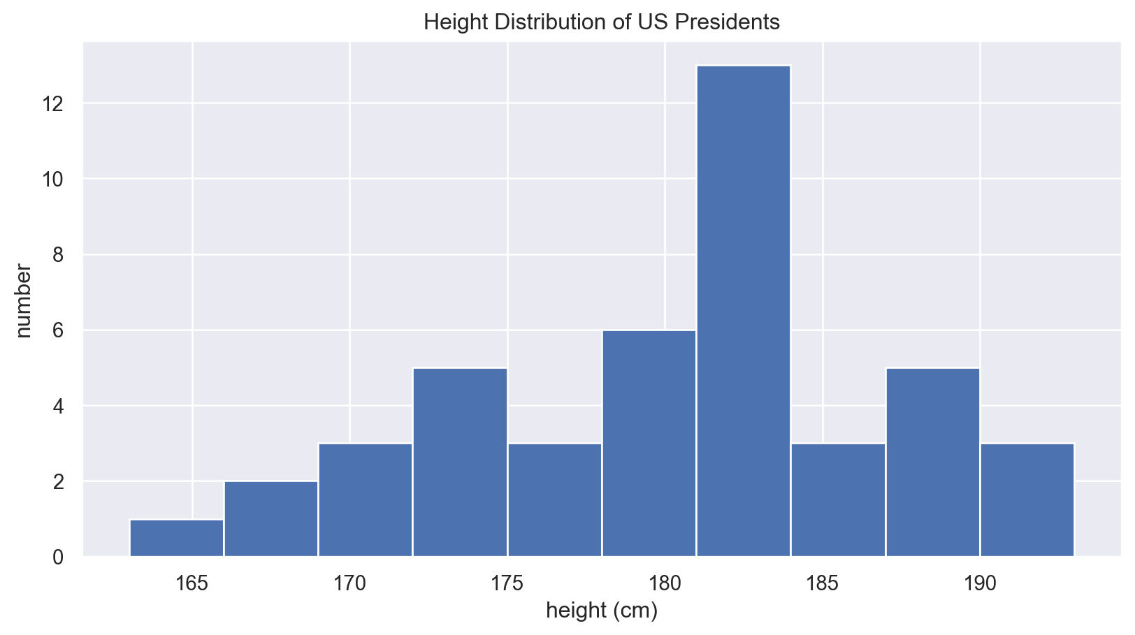
!pip3 install seaborn

Example: President Heights

• Uses a real-world dataset to demonstrate aggregates.

import numpy as np
import pandas as pd
data = pd.read_csv('https://raw.githubusercontent.com/jakevdp/PythonDataScienceHandbook/refs/heads/master/notebooks/data/president_heights.csv')
heights = np.array(data['height(cm)'])
print("Mean height: ", heights.mean())
print("Standard deviation:", heights.std())
print("Minimum height: ", heights.min())
print("Maximum height: ", heights.max())
print("25th percentile: ", np.percentile(heights, 25))
print("Median: ", np.median(heights))
print("75th percentile: ", np.percentile(heights, 75))

Mean height:  180.04545454545453
Standard deviation: 6.983599441335736
Minimum height:  163
Maximum height:  193
25th percentile:  174.75
Median:  182.0
75th percentile:  183.5

Visualizing President Heights

import matplotlib.pyplot as plt
import seaborn; seaborn.set()  # set plot style
plt.hist(heights)
plt.title('Height Distribution of US Presidents')
plt.xlabel('height (cm)')
plt.ylabel('number')
plt.plot()

Hands-on - Aggregations - 1/2

You’re a financial analyst tasked with analyzing historical stock data for several tech companies.

np.random.seed(42)
companies = ['TechCorp', 'DataSys', 'AIGlobal', 'CloudNet', 'CyberSec']
trading_days = 252
stock_data = np.random.randint(100, 200, size=(len(companies), trading_days))
stock_data = stock_data * (1 + np.random.randn(len(companies), trading_days) * 0.01)  # Add some randomness
print("Stock Data Shape:", stock_data.shape)
print("First six days of data:\n", stock_data[:, :6])

Stock Data Shape: (5, 252)
First six days of data:
 [[149.4074983  190.59940972 112.19491634 173.42047559 158.72559527
  120.79293028]
 [196.30842854 174.9778714  157.40229724 169.92405711 178.52343482
  191.48421877]
 [186.46131515 155.38937619 126.11957816 175.40848392 188.43959037
  169.95625021]
 [190.52887619 106.23981577 156.97119204 161.0857364  147.58640448
  124.25445626]
 [123.82077119 161.16804061 194.75072474 158.84621237 155.07543654
  159.51183387]]

Hands-on - Aggregations - 2/2

• Calculate for each company:
  • Average stock price
  • Highest and lowest stock prices
  • Standard deviation of stock prices
  • Number of days the stock price increased
    • Hint: np.diff
• Get the day with the highest average stock price across all companies
• Get the company with the most volatile stock (highest standard deviation)

NumPy

• Basic NumPy
• Universal Functions (UFuncs) in NumPy
• Aggregations
• Broadcasting
• Boolean Arrays and Masks

Broadcasting

Broadcasting: The Basic Idea

Enabling UFuncs to operate on arrays of different sizes

• Binary operations on arrays of the same size operate element-wise.

import numpy as np
a = np.array([0, 1, 2])
b = np.array([5, 5, 5])
print(a + b)

[5 6 7]

• Broadcasting allows operations on arrays of different sizes.

import numpy as np
a = np.array([0, 1, 2])
print(a + 5)

[5 6 7]

Broadcasting Analogy

“stretching” or “duplicating” the smaller array to match the shape of the larger array

Source

Broadcasting Example: Higher Dimensions

The 1D array a is “broadcast” across the 2nd dimension of M

import numpy as np
M = np.ones((3, 3))
a = np.arange(3)
print(M + a)

[[1. 2. 3.]
 [1. 2. 3.]
 [1. 2. 3.]]

Broadcasting Example: Both Arrays

Both a and b are broadcast to a common shape

import numpy as np
a = np.arange(3)
b = np.arange(3).reshape(3,1)  # Reshape b to be a column vector
print(a)
print(b)
print(a + b)

[0 1 2]
[[0]
 [1]
 [2]]
[[0 1 2]
 [1 2 3]
 [2 3 4]]

Rules of Broadcasting

• Rule 1: If the two arrays differ in their number of dimensions, the shape of the one with fewer dimensions is padded with ones on its leading (left) side.
• Rule 2: If the shape of the two arrays does not match in any dimension, the array with shape equal to 1 in that dimension is stretched to match the other shape.
• Rule 3: If in any dimension the sizes disagree and neither is equal to 1, an error is raised.

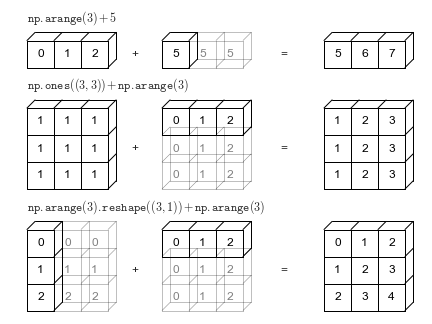
Broadcasting Example 1

import numpy as np
M = np.ones((2, 3))
a = np.arange(3)
print(M)
print(a)
print(M + a)

[[1. 1. 1.]
 [1. 1. 1.]]
[0 1 2]
[[1. 2. 3.]
 [1. 2. 3.]]

• Shapes:
  • M.shape = (2, 3)
  • a.shape = (3)

• Rule 1: Pad a with ones:
  • M.shape -> (2, 3)
  • a.shape -> (1, 3)
• Rule 2: Stretch the first dimension of a:
  • M.shape -> (2, 3)
  • a.shape -> (2, 3)
• Result: Shapes match!

Broadcasting Example 2

import numpy as np
a = np.arange(3).reshape((3, 1))
b = np.arange(3)
print(a)
print(b)
print(a + b)

[[0]
 [1]
 [2]]
[0 1 2]
[[0 1 2]
 [1 2 3]
 [2 3 4]]

• Shapes:
  • a.shape = (3, 1)
  • b.shape = (3)

• Rule 1: Pad b with ones (left):
  • a.shape -> (3, 1)
  • b.shape -> (1, 3)
• Rule 2: Stretch both arrays:
  • a.shape -> (3, 3)
  • b.shape -> (3, 3)
• Result: Shapes match!

Broadcasting Example 3: Incompatible

M = np.ones((3, 2))
a = np.arange(3)
print(M)
print(a)
# This will raise a ValueError:
# print(M + a)

[[1. 1.]
 [1. 1.]
 [1. 1.]]
[0 1 2]

• Shapes:
  • M.shape = (3, 2)
  • a.shape = (3,)
• 1: Pad a with ones:
  • M.shape -> (3, 2)
  • a.shape -> (1, 3)

• 2: Stretch the first dimension of a:
  • M.shape -> (3, 2)
  • a.shape -> (3, 3)
• 3: Shapes disagree, and neither dimension is 1. Error!

Broadcasting in Practice - 1

Centering an Array

X = np.random.random((10, 3))  # 10 observations, 3 features
print(X)

[[0.39543427 0.31320626 0.14706185]
 [0.4878512  0.13004778 0.83548024]
 [0.37039699 0.37480357 0.47400643]
 [0.44412771 0.99485797 0.54538112]
 [0.0882017  0.60687734 0.15158429]
 [0.03093764 0.97074215 0.77353889]
 [0.98010899 0.47787845 0.53225753]
 [0.16833696 0.24690743 0.83854921]
 [0.35618565 0.82681497 0.70901372]
 [0.17717093 0.50744637 0.67738732]]

Broadcasting in Practice - 2

Xmean = X.mean(0)  # Mean of each feature
print(Xmean)

[0.3498752  0.54495823 0.56842606]

X_centered = X - Xmean
print(X_centered.mean(axis=0))  # Should be near zero

[ 4.99600361e-17 -9.99200722e-17 -6.66133815e-17]

Broadcasting allows subtracting the feature means from each observation efficiently.

Hands-on - Broadcasting

You have temperature data for multiple cities over a week.

temperatures = np.random.randint(15, 35, size=(5, 7))
cities = ['New York', 'Los Angeles', 'Chicago', 'Houston', 'Phoenix']
days = ['Mon', 'Tue', 'Wed', 'Thu', 'Fri', 'Sat', 'Sun']
print(temperatures)

[[26 25 21 18 33 15 17]
 [27 29 16 25 18 33 31]
 [17 32 22 33 19 21 22]
 [19 31 19 18 33 16 25]
 [27 29 26 25 21 19 31]]

• Convert all temperatures from Celsius to Fahrenheit.
• Rank the temperatures for each day across cities (1 being the hottest, 5 being the coldest). np.argsort()
• Calculate a 3-day weighted moving average for each city, where the weights are [0.6, 0.3, 0.1] for [today, yesterday, day before yesterday]. np.dot()

NumPy

• Basic NumPy
• Universal Functions (UFuncs) in NumPy
• Aggregations
• Broadcasting
• Boolean Arrays and Masks

Boolean Arrays and Masks

Comparison Operators

import numpy as np
x = np.array([1, 2, 3, 4, 5])

print(x > 3)
print(x <= 3)
print(x == 3)
print(x != 3)

[False False False  True  True]
[ True  True  True False False]
[False False  True False False]
[ True  True False  True  True]

Rainfall Data: Create the Plot

rainfall = pd.read_csv('https://raw.githubusercontent.com/amankharwal/Website-data/refs/heads/master/Seattle2014.csv')['PRCP'].values
inches = rainfall / 254  # 1/10mm -> inches
plt.hist(inches, 40);
plt.xlabel("Inches")
plt.ylabel("Number of Days")
plt.show()

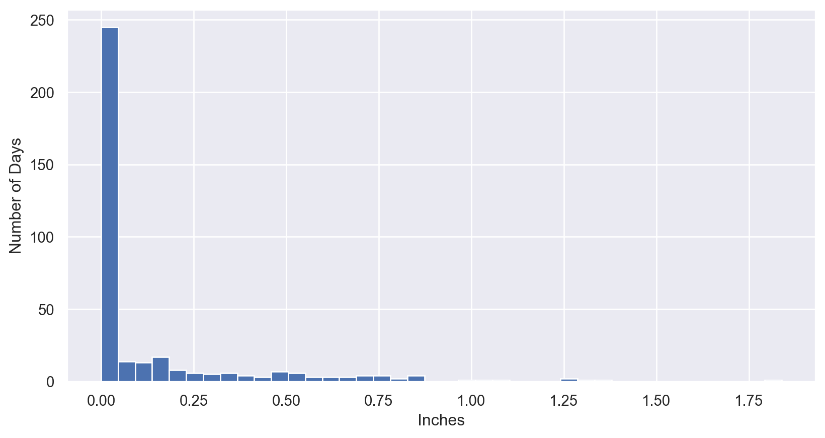
Rainfall Data: Boolean Masking

rainfall = pd.read_csv('https://raw.githubusercontent.com/amankharwal/Website-data/refs/heads/master/Seattle2014.csv')['PRCP'].values
inches = rainfall / 254  # 1/10mm -> inches
print("Number days without rain:      ", np.sum(inches == 0))
print("Number days with rain:         ", np.sum(inches != 0))
print("Days with more than 0.5 inches:", np.sum(inches > 0.5))
print("Rainy days with < 0.2 inches  :", np.sum((inches > 0) &
                                                (inches < 0.2)))

Number days without rain:       215
Number days with rain:          150
Days with more than 0.5 inches: 37
Rainy days with < 0.2 inches  : 75

any() and all()

• any(): Are any values True?
• all(): Are all values True?
• Can be used along axes, like aggregates.

rng = np.random.RandomState(0)
x = rng.randint(10, size=(3, 4))
print(np.any(x < 5))
print(np.all(x < 5))
print(np.any(x < 5, axis=1))
print(np.all(x < 5, axis=1))

True
False
[ True  True  True]
[False False False]

References

• Python Data Science Handbook

Questions?